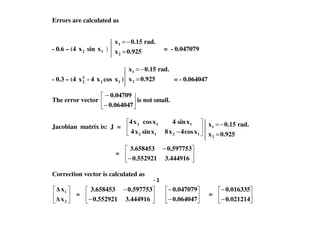
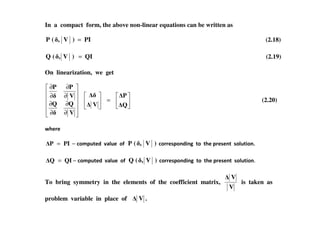
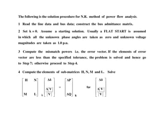
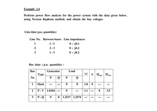
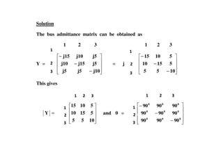
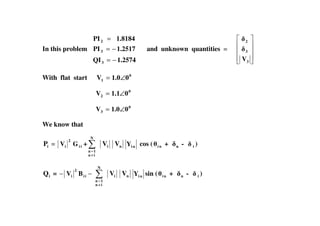
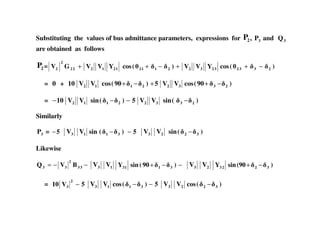
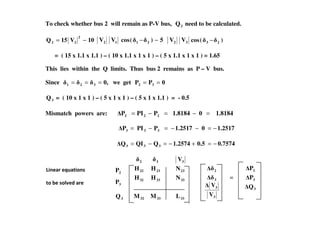
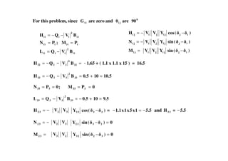
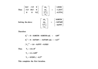
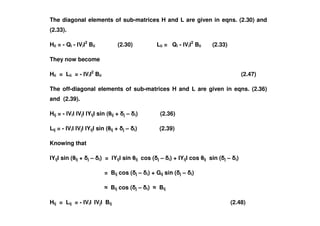
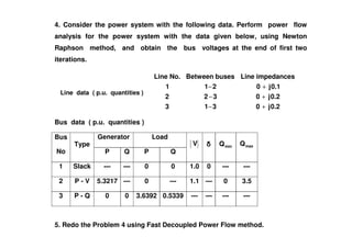
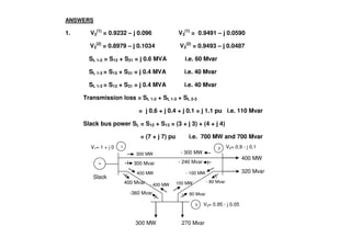
The document discusses power flow analysis, which determines bus voltages and power flows in a power system under normal steady-state operating conditions. It provides the mathematical formulation of the power flow problem as a set of nonlinear algebraic equations that must be solved iteratively. Buses are classified as slack, generator, or load buses depending on which two of four associated quantities - real power, reactive power, voltage magnitude, and voltage angle - are specified versus solved for. Solution methods like the Gauss-Seidel method are commonly used to iteratively solve the power flow equations until bus voltages converge.

2. FORMULATION OF POWER FLOW PROBLEM
Power flow analysis is the most fundamental study to be performed in a
power system both during the Planning and Operational phases. It
constitutes the major portion of electric utility. The study is concerned with
the normal steady state operation of power system and involves the
determination of bus voltages and power flows for a given network
configuration and loading condition.
The results of power flow analysis help to know
1 the present status of the power system, required for continuous
monitoring.
2 alternative plans for system expansion to meet the ever
increasing demand.
The mathematical formulation of the power flow problem results in a
system of non-linear algebraic equations and hence calls for an
iterative technique for obtaining the solution. Gauss-Seidel method and
Newton Raphson ( N.R.) method are the commonly used to get the power
flow solution.

3. With reasonable assumptions and approximations, a power system may
be modelled as shown in Fig. 2.1 for purpose of steady state analysis.
Static Capacitor
2
22 jQDPD +G
1
11 jQGPG +
11 jQDPD +
4
44 jQDPD +
3
G
33 δ∠V
33 jQGPG +
5
G
55 jQGPG +
Fig. 2.1 Typical power system network

4. The model consists of a network in which a number of buses are
interconnected by means of lines which may either transmission lines or
power transformers. The generators and loads are simply characterized
by the complex powers flowing into and out of buses respectively. Each
transmission line is characterized by a lumped impedance and a line
charging capacitance. Static capacitors or reactors may be located at
certain buses either to boost or buck the load-bus voltages at times ofcertain buses either to boost or buck the load-bus voltages at times of
need.
Thus the Power Flow problem may be stated as follows:
Given the network configuration and the loads at various buses,
determine a schedule of generation so that the bus voltages and hence
line flows remain within security limits.

5. A more specific statement of the problem will be made subsequently
after taking into consideration the following three observations.
1 For a given load, we can arbitrarily select the schedules of all the
generating buses, except one, to lie within the allowable limits of
the generation. The generation at one of the buses, called as the
slack bus, cannot be specified beforehand since the total generation
should be equal to the total demand plus the transmission losses,should be equal to the total demand plus the transmission losses,
which is not known unless all the bus voltages are determined.
2 Once the complex voltages at all the buses are known, all other
quantities of interest such as line flows, transmission losses and
generation at the buses can easily be determined. Hence the
foremost aim of the power flow problem is to solve for the bus
voltages.

6. 3 It will be convenient to use the Bus Power Specification which is
defined as the difference between the specified generation and load at
a bus. Thus for the kth bus, the bus power specification Sk is given by
Sk = PIk + j QIk
= (PGk + j QGk) - (PDk + j QDk)
= (PGk - PDk) + j (QGk - j QDk) (2.1)
In view of the above three observations Power Flow Problem may be
defined as that of determining the complex voltages at all the buses,
given the network configuration and the bus power specifications at all
the buses except the slack bus.

7. CLASSIFICATION OF BUSES
There are four quantities associated with each bus. They are PI, QI, V and .
Here PI is the real power injected into the bus
QI is the reactive power injected into the bus
V is the magnitude of the bus voltage
is the phase angle of the bus voltage
Any two of these four may be treated as independent variables ( i.e.
specified ) while the other two may be computed by solving the power
flow equations. Depending on which of the two variables are specified,flow equations. Depending on which of the two variables are specified,
buses are classified into three types. Three types of bus classification
based on practical requirements are shown below.
ss QI,PI ss ,V kk QI,PI kV k mm QI,PI mV m
? ? ? ? ? ?
Fig. 2.2 Three types of buses

8. Slack bus
In a power system with N buses, power flow problem is primarily concerned
with determining the 2N bus voltage variables, namely the voltage
magnitude and phase angles. These can be obtained by solving the 2N
power flow equations provided there are 2N power specifications.
However as discussed earlier the real and reactive power injection at the
SLACK BUS cannot be specified beforehand.
This leaves us with no other alternative but to specify two variables Vs
and arbitrarily for the slack bus so that 2( N-1 ) variables can beand s arbitrarily for the slack bus so that 2( N-1 ) variables can be
solved from 2( N-1 ) known power specifications.
Incidentally, the specification of Vs helps us to fix the voltage level of
the system and the specification of s serves as the phase angle reference
for the system.
Thus for the slack bus, both V and are specified and PI and QI
are to be determined. PI and QI can be computed at the end, when all
the V s and s are solved for.

9. Generator bus
In a generator bus, it is customary to maintain the bus voltage
magnitude at a desired level which can be achieved in practice by
proper reactive power injection. Such buses are termed as Voltage
Controlled Buses or P – V buses. At these buses PI and V are specified
and QI and are to be solved for.and QI and are to be solved for.
Load bus
The buses where there is no controllable generation are called as Load
Buses or P – Q buses. At the load buses, both PI and QI are specified
and V and are to be solved for.

10. POWER FLOW SOLUTION USING GAUSS SEIDEL METHOD
Development of power flow model
The power flow model will comprise of a set of simultaneous non-linear
algebraic equations. These equations relate the complex power injection
to complex bus voltages. The solution of this model will yield all the
bus voltages.
There are three types of equations namely
i) Network equations
ii) Bus power equations
iii) Line flow equations
The first two equations are used for the development of power flow
model. The solution of power flow model will yield all the bus voltages.
Once the bus voltages are known, the line and transformer flows can be
determined using the line flow equations.

11. Network equations
Network equations can be written in a number of alternative forms. Let
us choose the bus frame of reference in admittance form which is most
economical one from the point of view of computer time and memory
requirements.
The equations describing the performance of the network in the bus
admittance form is given by
I = Y V (2.2)
Here I is the bus current vector,
V is the bus voltage vector and
Y is the bus admittance matrix
In expanded form these equations are
N
2
1
I
I
I
=
NNN2N1
2N2221
1N1211
YYY
YYY
YYY
N
2
1
V
V
V
(2.3)

12. N
2
1
I
I
I
=
NNN2N1
2N2221
1N1211
YYY
YYY
YYY
N
2
1
V
V
V
(2.3)
Typical element of the bus admittance matrix is
Yij = |Yij |∠ ij = |Yij | cos ij + j |Yij | sin ij = Gij + j Bij (2.4)
Voltage at a typical bus i isVoltage at a typical bus i is
Vi = |Vi | ∠ i = |Vi | ( cos i + j sin i ) (2.5)
The current injected into the network at bus i is given by
n
N
1n
ni
nNi22i11ii
VY
VYVYVY
=
=
+++=I
(2.6)

13. Bus power equations
In addition to the linear network equations given by eqn. (2.3), bus
power equations should also be satisfied in power flow problem. These
bus power equations introduce non- linearity into the power flow model.
The complex power entering at the th
k bus is given by
*
kkkk VQjP I=+ (2.7)
This power should be the same as the bus power specification. Thus
we have
*
=+ *
kkkk VQIjPI I=+ (2.8)
sk
N,1,2,k
≠
=
Equations (2.6) and (2.8) can be suitably combined to obtain the power
flow model.
The following two methods are used to solve the power flow model.
1. Gauss-Seidel method
2. Newton Raphson method

14. Gauss-Seidel method
Gauss-Seidel method is used to solve a set of algebraic equations.
Consider
NNNN2N21N1
2N2N222121
1N1N212111
yxaxaxa
yxaxaxa
yxaxaxa
=+++
=+++
=+++
Specifically
xayxaThus
yxaxaxaxa
N
km
1m
mkmkkkk
kNkNkkk2k21k1
−=
=+++++
≠
=
N,1,2,k
xay
a
1
xgivesThis m
N
km
1m
kmk
kk
k
=
−=
≠
=
Initially, values of N21 x,,x,x are assumed. Updated values are calculated
using the above equation. In any iteration 1h + , up to ,1km −= values of mx
calculated in 1h + iteration are used and for 1km += to N , values of
mx calculated in h iteration are used. Thus
−−=
−
= +=
++
1k
1m
N
1km
h
mkm
1h
mkmk
kk
1h
k xaxay
a
1
x (2.9)

15. Gauss-Seidel method for power flow solution
In this method, first an initial estimate of bus voltages is assumed. By
substituting this estimate in the given set of equations, a second
estimate, better than the first one, is obtained. This process is repeated
and better and better estimates of the solution are obtained until the
difference between two successive estimates becomes lesser than a
prescribed tolerance.
Let us now find the required equations for calculating the bus voltages.
From the network equations, we have
m
N
km
1m
kmkkkm
N
1m
kmk
NkNkkk2k21k1k
VYVYVYThus
VYVYVYVY
≠
==
+==
+++++=
I
I
(2.10)

16. From the bus power specifications, we have
sk
N,1,2,kforVQIjPI *
kkkk
≠
==+ I
kI is the intermediate variable. This can be eliminated. Taking conjugate of
above equation
*
k
kk
kk
*
kkk
V
QIjPI
Therefore;VQIjPI
−
==− II (2.12)
From equations (2.10) and (2.12) we get
N
QIjPI −
(2.11)
=+
≠
=
m
N
km
1m
kmkkk VYVY *
k
kk
V
QIjPI −
sk
N,1,2,k
V
Y
Y
V
1
Y
QIjPI
sk
N,1,2,k
VY
V
jQIPI
Y
1
VThus
m
N
km
1m kk
km
*
kkk
kk
N
km
1m
mkm*
k
kk
kk
k
≠
=
−
−
=
≠
=
−
−
=
≠
=
≠
=
(2.13)

17. A significant reduction in computing time for a solution can be achieved
by performing as many arithmetic operations as possible before initiating
the iterative calculation. Let us define
k
kk
kk
A
Y
QIjPI
=
−
(2.14)
km
kk
km
B
Y
Y
and = (2.15)
Having defined kmk BandA equation (2.13) becomes
skN,1,2,kVB
V
A
V
N
km
1m
mkm*
k
k
k ≠=−=
≠
=
(2.16)
When Gauss-Seidel iterative procedure is used, the voltage at the th
k
bus during th
1h + iteration, can be computed as
sk
N,1,2,k
VBVB
V
A
V
N
1km
h
mkm
1k
1m
1h
mkm*h
k
k1h
k
≠
=
−−=
+=
−
=
++
(2.17)

18. yk0
ikm
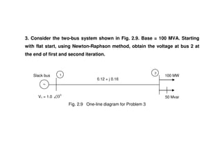
ym0
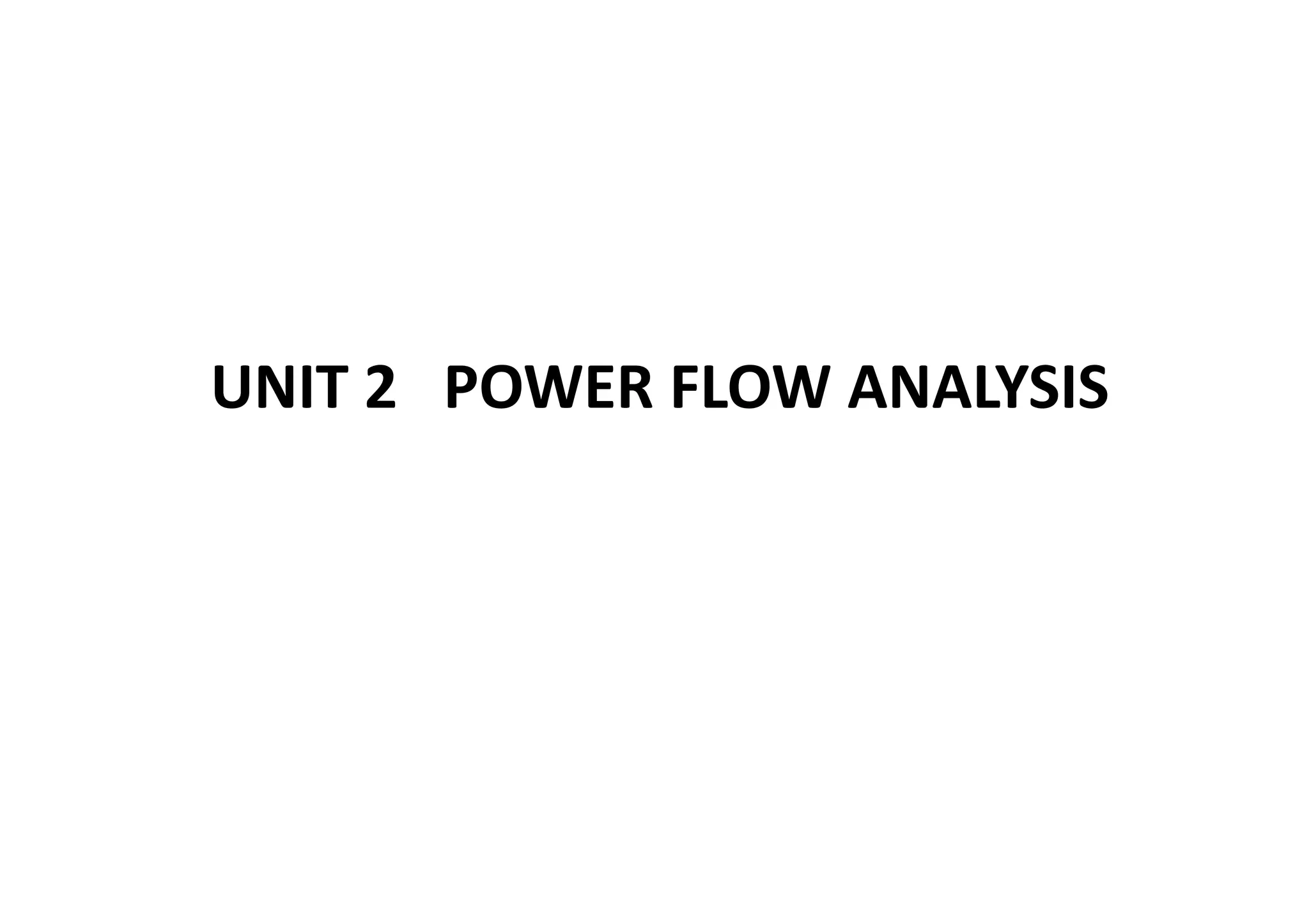
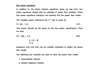
Line flow equations
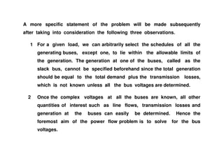
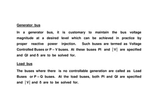
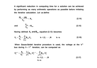
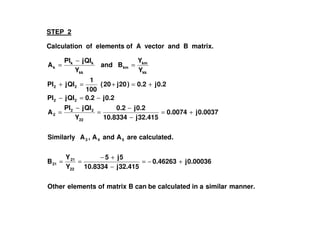
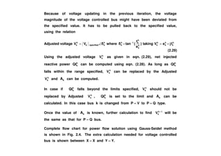
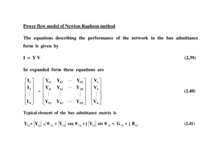
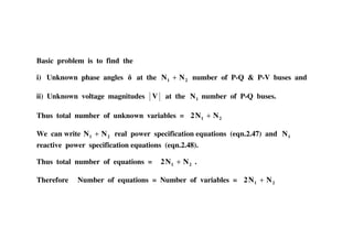
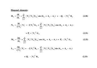
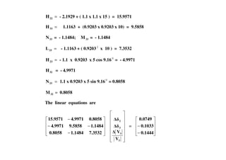
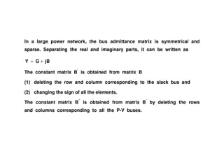
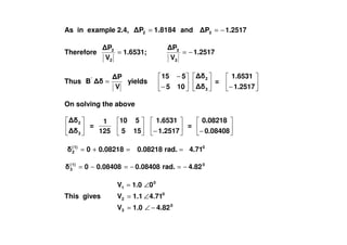
Knowing the bus voltages, the power in the lines can be computed as
shown below.
k0kkmmkkm yVy)VV(Current +−=i
(2.18)
Power flow from bus k to bus mis *
kmkkm VS i= (2.19)
Fig. 2.3 Circuit for
line flow calculation
ykm
Substituting equation (2.18) in equation (2.19)
]yVy)VV([VS *
k0
*
k
*
km
*
m
*
kkkm +−= (2.20)
Similarly, power flow from bus m to bus k is
]yVy)VV([VS *
m0
*
m
*
km
*
k
*
mmmk +−= (2.21)
The line loss in the transmission line mk − is given by
mkkmmkL SSS +=− (2.22)
Total transmission loss in the system is
−
−=
linesthe
allover
ji
jiLL SS (2.23)

19. Example 2.1
For a power system, the transmission line impedances and the line charging
admittances in p.u. on a 100 MVA base are given in Table 1. The scheduled
generations and loads on different buses are given in Table 2. Taking the slack
bus voltage as 1.06 + j 0.0 and using a flat start perform the power flow
analysis and obtain the bus voltages, transmission loss and slack bus power.
Table 1 Transmission line data:
Sl. No.
Bus code
k - m
Line Impedance
kmz HLCA
1 1 – 2 0.02 + j 0.06 j 0.030
2 1 – 3 0.08 + j 0.24 j 0.025
3 2 – 3 0.06 + j 0.18 j 0.0203 2 – 3 0.06 + j 0.18 j 0.020
4 2 – 4 0.06 + j 0.18 j 0.020
5 2 – 5 0.04 + j 0.12 j 0.015
6 3 – 4 0.01 + j 0.03 j 0.010
7 4 – 5 0.08 + j 0.24 j 0.025
Table 2 Bus data:
Bus code
k
Generation Load
RemarkMWinkPG MVARinkQG MWinkPD MVARinkQD
1 --- --- 0 0 Slack bus
2 40 30 20 10 P – Q bus
3 0 0 45 15 P – Q bus
4 0 0 40 5 P – Q bus
5 0 0 60 10 P – Q bus

20. Solution
Flat start means all the unknown voltage magnitude are taken as 1.0 p.u.
and all unknown voltage phase angles are taken as 0.
Thus initial solution is
0j1.0VVVV
0j1.06V
(0)
5
(0)
4
(0)
3
(0)
2
1
+====
+=
STEP 1
For the transmission system, the bus admittance matrix is to be calculated.
Sl.
No.
Bus
code
Line Impedance
z
Line admittance
y
HLCA
No.
code
k - m kmz ykm
HLCA
1 1 – 2 0.02 + j 0.06 5 - j 15 j 0.030
2 1 – 3 0.08 + j 0.24 1.25 – j 3.75 j 0.025
3 2 – 3 0.06 + j 0.18 1.6667 – j 5 j 0.020
4 2 – 4 0.06 + j 0.18 1.6667 – j 5 j 0.020
5 2 – 5 0.04 + j 0.12 2.5 – j 7.5 j 0.015
6 3 – 4 0.01 + j 0.03 10 – j 30 j 0.010
7 4 – 5 0.08 + j 0.24 1.25 – j 3.75 j 0.025
Y22 = (5 – j15) + (1.6667 – j5) + (1.6667 – j5) + (2.5 – j7.5) + j 0.03 + j 0.02 + j 0.02 + j 0.015
= 10.8334 – j 32.415
Similarly Y33 = 12.9167– j 38.695 Y44 = 12.9167 – j 38.695 ; Y55 = 3.75 – j 11.21

21. ! !
! !

22. STEP 2
Calculation of elements of A vector and B matrix.
0.0037j0.0074
0.2j0.2QIjPI
A
0.2j0.2QIjPI
0.2j0.2)20j20(
100
1
QIjPI
Y
Y
Band
Y
QIjPI
A
22
2
22
22
kk
km
km
kk
kk
k
+=
−
−
=
−
=
−=−
+=+=+
=
−
=
manner.similaraincalculatedbecanBmatrixofelementsOther
0.00036j0.46263
32.415j10.8334
5j5
Y
Y
B
.calculatedareAandA,ASimilarly
0.0037j0.0074
32.415j10.8334Y
A
22
21
21
543
22
2
+−=
−
+−
==
+=
−
==

23. Thus
! !
!
"
! ! !
! ! !

24. STEP 3
Iterative computation of bus voltage can be carried out as shown.
New estimate of voltage at bus 2 is calculated as:
)00.0j1.06()0.00036j0.46263(
0j1.0
0.00370j0.00740
VBVBVBVB
V
A
V )0(
525
)0(
424
)0(
323121*)0(
2
2)1(
2
++−−
−
+
=
−−−−=
0.00290j1.03752
)0.0j1.0()0.00018j0.23131(
)0.0j1.0()0.00012j0.15421()0.0j1.0()0.00012j0.15421(
0j1.0
+=
++−−
++−−++−−
−
This value of voltage V2
(1)
will replace the previous value of voltage V2
(0)
before doing subsequent calculations of voltages.

25. This value of voltage V2
(1)
will replace the previous value of voltage V2
(0)
before doing subsequent calculations of voltages.
The rate of convergence of the iterative process can be increased by
applying an ACCELERATION FACTOR to the approximate solution
obtained. For example on hand, from the estimate V2
(1)
we get the
change in voltage
V2 = V2
(1)
– V2
(0)
= (1.03753 + j 0.00290) – (1.0 + j 0) = 0.03752 + j 0.00290
The accelerated value of the bus voltage is obtained as V2
(1)
= V2
(0)
+ V2
By assuming = 1.4 accelerated bus voltage
V2
(1)
= (1.0 + j 0) + 1.4 (0.03752 + j 0.00290) = 1.05253 + j 0.00406
This new value of voltage V2
(1)
will replace the previous value of the bus
voltage V2
(0)
and is used in the calculation of voltages for the remaining
buses. In general
Vk
h+1
accld = Vk
h
+ (Vk
h+1
– Vk
h
) (2.24)
where k is the bus at which the voltage is calculated and h+1 is the current
iteration count.

26. The process is continued for the remaining buses to complete one
iteration. For the next bus 3
0.00921j1.00690
)0j1.0()0.00033j0.77518(
)0.00406j1.05253()0.00006j0.12920(
)0j1.06()0.00004j0.09690(
0j1.0
0.00930j0.00698
VBVBVB
V
A
V )0(
434
)1(
232131*)0(
3
3)1(
3
−=
++−−
++−−
++−−
−
−−
=
−−−=
The accelerated value can be calculated as
V3
h+1
accld = V3
h
+ (V3
h+1
– V3
h
) = (1.0 + j 0) + 1.4 (0.00690 – j 0.00921)V3
h+1
accld = V3
h
+ (V3
h+1
– V3
h
) = (1.0 + j 0) + 1.4 (0.00690 – j 0.00921)
= 1.00966 – j 0.01289
Continuing this process of calculation, at the end of first iteration, the
bus voltages are obtained as
V1 = 1.06 + j 0.0 V2
(1)
= 1.05253 + j 0.00406 V3
(1)
= 1.00966 – j 0.01289
V4
(1)
= 1.01599 – j 0.02635 V5
(1)
= 1.02727 – j 0.07374
If and are the acceleration factors for the real and imaginary components
of voltages respectively, the accelerated values can be computed as
ek
h+1
= ek
h
+ (ek
h+1
- ek
h
) fk
h+1
= fk
h
+ (fk
h+1
- fk
h
) (2.25)

27. Convergence
The iterative process must be continued until the magnitude of change
of bus voltage between two consecutive iterations is less than a certain
level for all bus voltages. We express this in mathematical form as
Vmax = max. of |Vk
h+1
– Vk
h
| for k = 1,2, …… , N k s
and Vmax <
If 1 and 2 are the tolerance level for the real and imaginary parts of
bus voltages respectively, then the convergence criteria will be
(2.26)
Vmax 1 = max. of |ek
h+1
– ek
h
| Vmax 2 = max. of |fk
h+1
– fk
h
|
for k = 1,2, …… , N k s
Vmax 1 < 1 and Vmax 2 < 2
For the problem under study 1 = 2 = 0.0001
The final converged bus voltages obtained after 10 iterations are given below.
V1 = 1.06 + j 0.0 V2 = 1.04623 - j 0.05126 V3 = 1.02036 – j 0.08917
V4 = 1.01920 – j 0.09504 V5 = 1.01211 – j 0.10904
(2.35)(2.27)

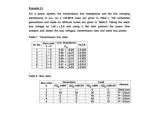
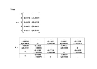
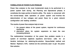
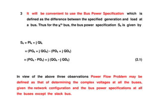
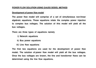
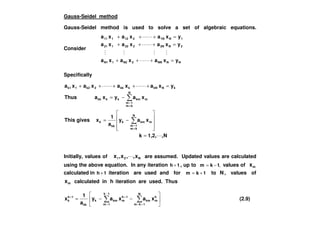
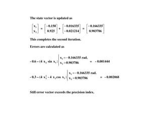
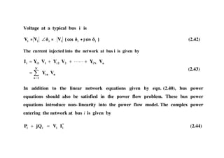
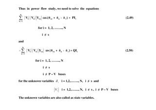
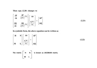
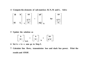
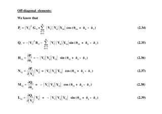
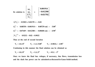
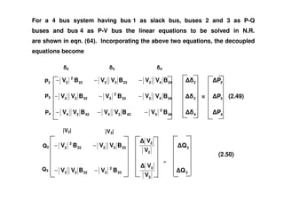
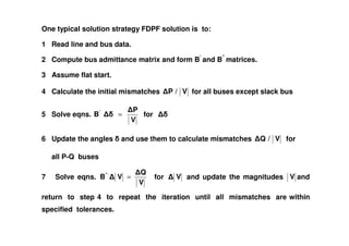
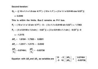
28. Computation of line flows and transmission loss
Line flows can be computed from
)0.086j0.888(
]})0.03j0.0(0)j1.06({
)15j5(})0.05126j1.04623()0j1.06({[)0j(1.06
]yVy)VV([VS
]yVy)VV([VS
*
10
*
1
*
12
*
2
*
1112
*
k0
*
k
*
km
*
m
*
kkkm
−=
−−+
++−−+=
+−=
+−=
)0.086j0.888( −=
)0.062j0.874(
]})0.03j(0.0)0.05126j1.04623({
15)j5}()0j1.06(0.05126)j1.04623({[)0.05126j1.04623(
yVy)VV([VS
Similarly
*
20
*
2
*
12
*
1
*
2221
+−=
−++
+−−+−=
+−=

29. Power loss in line 1 – 2 is
)0.024j0.014(
0.062)j0.874(0.086)j(0.888SSS 211221L
−=
+−+−=+=−
Power loss in other lines can be computed as
0.029j0.004S
0.033j0.004S
0.019j0.012S
42L
32L
31L
−=
−=
−=
−
−
−
0.051j0.0S
0.019j0.0S
0.002j0.011S
0.029j0.004S
54L
43L
52L
42L
−=
−=
+=
−=
−
−
−
−
Total transmission loss SL = ( 0.045 - j 0.173 ) i.e.
Real power transmission loss = 4.5 MW
Reactive power transmission loss = 17.3 MVAR ( Capacitive )

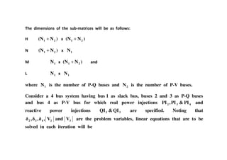
30. S ds
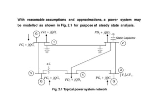
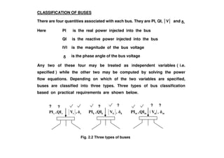
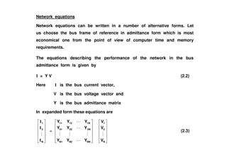
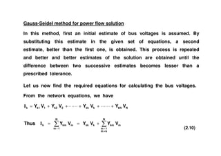
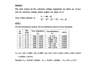
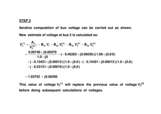
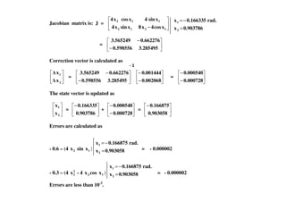
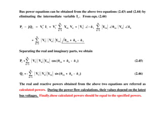
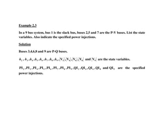
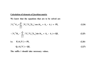
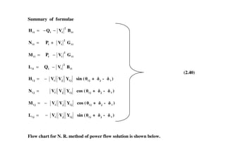
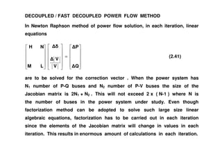
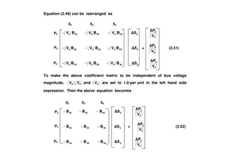
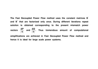
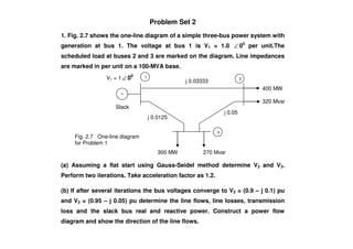
Computation of slack bus power
Slack bus power can be determined by summing up the powers flowing
out in the lines connected at the slack bus and the load at the slack bus.
S13
S gs
S12
In this case, load at slack bus is zero and hence slack bus power is
1213gs SSS +=
)0.011j0.407(
]})0.025j0.0(0)j1.06({
)3.75j1.25(})0.08917j1.02036()0j1.06({[)0j(1.06
]yVy)VV([VS *
10
*
1
*
13
*
3
*
1113
+=
−−+
++−−+=
+−=
)0.075j1.295()0.086j0.888()0.011j0.407(SSS 1213gs −=−++=+=
Thus the power supplied by the slack bus:
Real power = 129.5 MW Reactive power = 7.5 MVAR (Capacitive )

31. Voltage controlled bus
In voltage controlled bus k net real power injection kPI and voltage
magnitude kV are specified. Normally minmax QIandQI will also be
specified for voltage controlled bus. Since kQI is not known, kA given
by
kk
kk
Y
QIjPI −
cannot be calculated. An expression for kQI can be
developed as shown below.
We know k
*
kkk
*
kkkkm
N
1m
mkk IVQIjPIi.e.IVQIjPIandVY =−=+=
=
I
Denoting haveweVVandYY iiijijiji ∠=∠=
=
==
−+−=
−+=+∠−∠=−
N
1m
kmmkmkmkk
kmmkmk
N
1m
mkmmkm
N
1m
mkkkkk
sinYVVQIThus
YVVVYVQIjPI
The value of kV to be used in equation (2.28) must satisfy the
relation
specifiedkk VV =
(2.28)

32. Because of voltage updating in the previous iteration, the voltage
magnitude of the voltage controlled bus might have been deviated from
the specified value. It has to be pulled back to the specified value,
using the relation
Adjusted voltage h
k
h
k
h
kh
k
h
k1h
k
h
kspecifiedk
h
k fjeVtaking)
e
f
(tanwhereVV +==∠= −
Using the adjusted voltage h
kV as given in eqn. (2.29), net injected
reactive power h
kQI can be computed using eqn. (2.28). As long as h
kQI
falls within the range specified, h
kV can be replaced by the Adjusted
h
V and A can be computed.
(2.29)
h
kV and kA can be computed.
In case if h
kQI falls beyond the limits specified, h
kV should not be
replaced by Adjusted h
kV , h
kQI is set to the limit and kA can be
calculated. In this case bus k is changed from P – V to P – Q type.
Once the value of kA is known, further calculation to find 1h
kV +
will be
the same as that for P – Q bus.
Complete flow chart for power flow solution using Gauss-Seidel method
is shown in Fig. 2.4. The extra calculation needed for voltage controlled
bus is shown between X – X and Y – Y.

33. START
READ LINE DATA & BUS DATA
FORM Y MATRIX
ASSUME skNkVk ≠= ,,2,1)0(
COMPUTE kA FOR P – Q BUSES
COMPUTE kmB SET h = 0
SET k = 1 AND 0.0=∆ MAXV
k : s YES
X -------------------------------------------- NO-----------------------------------------
NO k : V.C. Bus X
YES
COMPUTE
h
kδ ADJUSTED VOLTAGE,
h
kQI
≤ ≥
MAXk
h
k QIQI : MINk
h
k QIQI :
> <
REPLACE
h
kQI BY MAXkQI REPLACE
h
kQI BY MINkQI REPLACE
h
kV BY ADJ
h
kVkQI MAXkQI kQI MINkQI kV kV
Y COMPUTE kA Y
-----------------------------------------------------------------------------------------------------------------
COMPUTE ;1+h
kV COMPUTE
h
k
h
k VVV −=∆ +1
YES
MAXVV ∆≥∆ SET VVMAX ∆=∆
NO
REPLACE
h
kV BY
1+h
kV
SET k = k + 1
k : N IS MAXV∆ <ε YES
NO
SET h = h + 1
COMPUTE LINE FLOWS, SLACK BUS POWER
PRINT THE RESULTS
STOP
≤
>

34. Introduction
Gauss-Seidel method of solving the power flow has simple problem formulation and
hence easy to explain However, it has poor convergence characteristics. It takes large
number of iterations to converge. Even for the five bus system discussed in Example 2.1,
it takes 10 iterations to converge.
Newton Raphson (N.R.) method of solving power flow is based on the Newton Raphson
method of solving a set of non-linear algebraic equations. N. R. method of solving power
flow problem has very good convergence characteristics. Even for large systems it takes
only two to four iterations to converge.only two to four iterations to converge.
Newton Raphson method of solving a set of non-linear equations
Let the non-linear equations to be solved be
1k)x,,x,(xf n211 =
2n212 k)x,,x,(xf =
nn21n k)x,,x,(xf =

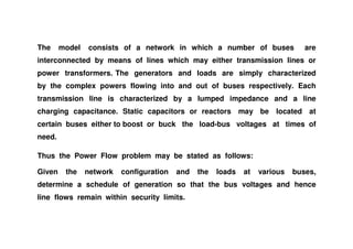
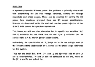
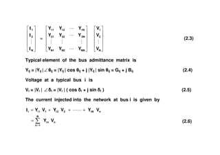
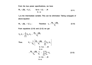
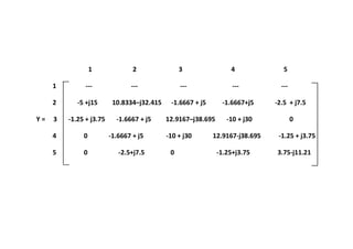
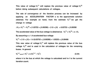
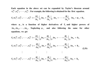
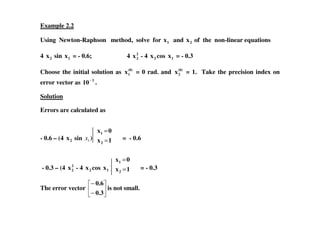
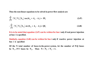
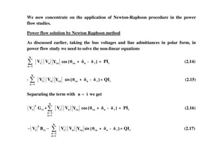
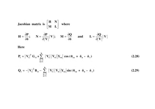
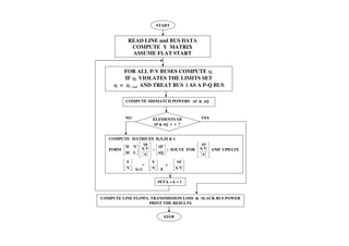
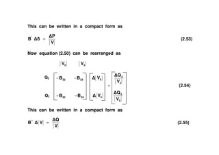
35. Let the initial solution be (0)
n
(0)
2
(0)
1 x,,x,x
If 0)x,,x,(xfk (0)
n
(0)
2
(0)
111 −
0)x,,x,(xfk (0)
n
(0)
2
(0)
122 −
0)x,,x,(xfk (0)
n
(0)
2
(0)
1nn −
then the solution is reached. Let us say that the solution is not reached. Assume
n21 x,,x,x are the corrections required on (0)
n
(0)
2
(0)
1 x,,x,x respectively.
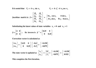
Then
1k)]x(x,),x(x),x[(xf n
(0)
n2
(0)
21
(0)
11 =+++
2n
(0)
n2
(0)
21
(0)
12 k)]x(x,),x(x),x[(xf =+++
(2.30)
nn
(0)
n2
(0)
21
(0)
1n k)]x(x,),x(x),x[(xf =+++

36. Each equation in the above set can be expanded by Taylor’s theorem around
(0)
n
(0)
2
(0)
1 x,,x,x . For example, the following is obtained for the first equation.
(0)
n
(0)
2
(0)
11 x,,x,(xf
1
1
x
f
)
∂
∂
+
2
1
1
x
f
x
∂
∂
+
n
1
2
x
f
x
∂
∂
++ 11n kx =+
where 1 is a function of higher derivatives of 1f and higher powers of
n21 x,,x,x . Neglecting 1 and also following the same for other
equations, we get
f∂ f∂ f∂(0)
n
(0)
2
(0)
11 x,,x,(xf
1
1
x
f
)
∂
∂
+
2
1
1
x
f
x
∂
∂
+
n
1
2
x
f
x
∂
∂
++ 1n kx =
(0)
n
(0)
2
(0)
12 x,,x,(xf
1
2
x
f
)
∂
∂
+
2
2
1
x
f
x
∂
∂
+
n
2
2
x
f
x
∂
∂
++ 2n kx =
(0)
n
(0)
2
(0)
1n x,,x,(xf
1
n
x
f
)
∂
∂
+
2
n
1
x
f
x
∂
∂
+
n
n
2
x
f
x
∂
∂
++ nn kx =
(2.31)

37. (2.32)
The matrix form of equations (2.31) is
)x,,x,x(fkx
x
f
x
f
x
f (0)
n
(0)
2
(0)
1111
n
1
2
1
1
1
−
∂
∂
∂
∂
∂
∂
)x,,x,x(fkx
x
f
x
f
x
f (0)
n
(0)
2
(0)
1222
n
2
2
2
1
2
−
∂
∂
∂
∂
∂
∂
)x,,x,x(fkx
x
f
x
f
x
f (0)
n
(0)
2
(0)
1nnn
n
n
2
n
1
n
−
∂
∂
∂
∂
∂
∂
The above equation can be written in a compact form as
)X(FKX)X(F (0)(0)'
−= (2.33)

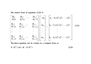
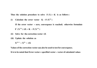
38. The above equation can be written in a compact form as
)X(FKX)X(F (0)(0)'
−= (2.33)
This set of linear equations need to be solved for the correction vector
=
n
2
1
x
x
x
X
)X(FKX)X(F (0)(0)'
−= (2.34)
In eqn.(1.50) )X(F (0)'
is called the JACOBIAN MATRIX and the vector
)X(FK (0)
− is called the ERROR VECTOR. The Jacobian matrix is also denoted as J.
Solving eqn. (2.34) for X
X = [ ] 1)0('
)X(F −
[ ])X(FK )(0
− (2.35)

39. Then the improved estimate is
XXX )0(1)(
+=
Generalizing this, for th
)1h( + iteration
XXX )h()1h(
+=+
where (2.36)XXX += where (2.36)
[ ] [ ])X(FK)X(FX )h(1)h('
−= −
(2.37)
i.e. X is the solution of )X(FKX)X(F )h()h('
−= (2.38)

40. Thus the solution procedure to solve K)X(F = is as follows :
(i) Calculate the error vector )X(FK (h)
−
If the error vector ≈ zero, convergence is reached; otherwise formulate
)X(FKX)X(F (h)(h)'
−=
(ii) Solve for the correction vector X(ii) Solve for the correction vector X
(iii) Update the solution as
XXX (h)1)(h
+=+
Values of the correction vector can also be used to test for convergence.
It is to be noted that Error vector = specified vector – vector of calculated values

41. Example 2.2
Using Newton-Raphson method, solve for 1x and 2x of the non-linear equations
4 2x sin 1x = - 0.6; 4 2
2x - 4 2x cos 1x = - 0.3
Choose the initial solution as (0)
1x = 0 rad. and (0)
2x = 1. Take the precision index on
error vector as 3
10−
.
Solution
Errors are calculated asErrors are calculated as
- 0.6 – (4 2x sin 1x ) = - 0.6
- 0.3 – (4 2
2x - 4 2x cos 1x ) = - 0.3
The error vector
−
−
0.3
0.6
is not small.
1x
0x
2
1
=
=
1x
0x
2
1
=
=

42. It is noted that 1f = 4 2x sin 1x 2f = 4 2
2x - 4 2x cos 1x
Jacobian matrix is: J =
∂
∂
∂
∂
∂
∂
∂
∂
2
2
1
2
2
1
1
1
x
f
x
f
x
f
x
f
=
− 1212
112
xcos4x8xsinx4
xsin4xcosx4
Substituting the latest values of state variables 1x = 0 and 2x = 1
J =
40
04
; Its inverse is 1
J−
=
0.250
00.25
40 0.250
Correction vector is calculated as
2
1
x
x
=
0.250
00.25
−
−
0.3
0.6
=
−
−
0.075
0.150
The state vector is updated as
2
1
x
x
=
1
0
+
−
−
0.075
0.150
=
−
0.925
0.150
This completes the first iteration.

43. Errors are calculated as
- 0.6 – (4 2x sin 1x ) = = - 0.047079
- 0.3 – (4 2
2x - 4 2x cos 1x ) = - 0.064047
The error vector
−
−
0.064047
0.04709
is not small.
0.925x
rad.0.15x
2
1
=
−=
0.925x
rad.0.15x
2
1
=
−=
Jacobian matrix is: J =
− 1212
112
xcos4x8xsinx4
xsin4xcosx4
=
−
−
3.4449160.552921
0.5977533.658453
Correction vector is calculated as
2
1
x
x
=
−
−
3.4449160.552921
0.5977533.658453
−
−
0.064047
0.047079
=
−
−
0.021214
0.016335
0.925x
rad.0.15x
2
1
=
−=

44. The state vector is updated as
2
1
x
x
=
−
0.925
0.150
+
−
−
0.021214
0.016335
=
−
0.903786
0.166335
This completes the second iteration.
Errors are calculated as
rad.0.166335x −=
- 0.6 – (4 2x sin 1x ) = = - 0.001444
- 0.3 – (4 2
2x - 4 2x cos 1x ) = - 0.002068
Still error vector exceeds the precision index.
0.903786x
rad.0.166335x
2
1
=
−=
0.903786x
rad.0.166335x
2
1
=
−=

45. Jacobian matrix is: J =
− 1212
112
xcos4x8xsinx4
xsin4xcosx4
=
−
−
3.2854950.598556
0.6622763.565249
Correction vector is calculated as
2
1
x
x
=
−
−
3.2854950.598556
0.6622763.565249
−
−
0.002068
0.001444
=
−
−
0.000728
0.000540
The state vector is updated as
0.903786x
rad.0.166335x
2
1
=
−=
2
1
x
x
=
−
0.903786
0.166335
+
−
−
0.000728
0.000540
=
−
0.903058
0.166875
Errors are calculated as
- 0.6 – (4 2x sin 1x ) = = - 0.000002
- 0.3 – (4 2
2x - 4 2x cos 1x ) = - 0.000002
Errors are less than 10-3
.
0.903058x
rad.0.166875x
2
1
=
−=
0.903058x
rad.0.166875x
2
1
=
−=

46. The final values of 1x and 2x are - 0.166875 rad. and 0.903058 respectively.
The results can be checked by substituting the solution in the original equations:
4 2x sin 1x = - 0.6 4 2
2x - 4 2x cos 1x = - 0.3
In this example, we have actually solved our first power flow problem by N.R. method.
This is because the two non-linear equations of this example are the power flow model
of the simple system shown in Fig. 2.5 below.
# $
1V 1∠ 2V 2∠
Here bus 1 is the slack bus with its voltage 1V 1∠ = 1.0 0
0∠ p.u. Further 1x
represents the angle 2 and 2x represents the voltage magnitude 2V at bus 2.
p.u.)0.3j0.6(QP 2d2d +=+
# $
%
&' ( ) *$++,+-./

47. Power flow model of Newton Raphson method
The equations describing the performance of the network in the bus admittance
form is given by
I = Y V (2.39)
In expanded form these equations are
N
2
1
I
I
I
NNN2N1
2N2221
1N1211
YYY
YYY
YYY
N
2
1
V
V
V
(2.40)
Typical element of the bus admittance matrix is
jiY jiY ji∠ jiY 0)+ ji jiY +&1 ji jiG jiB (2.41)

48. Voltage at a typical bus i is
iV iV i∠ iV 20)+ i +&1 i 3 (2.42)
The current injected into the network at bus i is given by
n
N
1n
ni
nNi22i11ii
VY
VYVYVYI
=
=
+++=
(2.43)
1n =
In addition to the linear network equations given by eqn. (2.40), bus power
equations should also be satisfied in the power flow problem. These bus power
equations introduce non- linearity into the power flow model. The complex power
entering the network at bus i is given by
*
iiii IVQjP =+ (2.44)

49. Bus power equations can be obtained from the above two equations (2.43) and (2.44) by
eliminating the intermediate variable iI . From eqn. (2.44)
iIVQjP *
iii =− *
iV n
N
1n
ni VY
=
iV i−∠
=
N
1n
niY ni∠ nV n∠
=
N
1n
iV nV niY ni n i
Separating the real and imaginary parts, we obtain
N
iP
=
N
1n
iV nV niY 0)+2 ni n i 3 (2.45)
iQ
=
N
1n
iV nV niY +&1 2 ni n i 3 (2.46)
The real and reactive powers obtained from the above two equations are referred as
calculated powers. During the power flow calculations, their values depend on the latest
bus voltages. Finally,these calculated powers should be equal to the specified powers.

50. Thus the non-linear equations to be solved in power flow analysis are
=
N
1n
iV nV niY 0)+2 ni n i 3 iPI (2.47)
=
N
1n
iV nV niY +&1 2 ni n i 3 iQI (2.48)
It is to be noted that equation (2.47) can be written for bus i only if real power injectionIt is to be noted that equation (2.47) can be written for bus i only if real power injection
at bus i is specified.
Similarly, equation (2.48) can be written for bus i only if reactive power injection at
bus i is specified.
Of the N total number of buses in the power system, let the number of P-Q buses
be 1N , P-V buses be 2N . Then 1NNN 21 ++= .

51. Basic problem is to find the
i) Unknown phase angles at the 21 NN + number of P-Q & P-V buses and
ii) Unknown voltage magnitudes V at the 1N number of P-Q buses.
Thus total number of unknown variables = 21 NN2 +
We can write 21 NN + real power specification equations (eqn.2.47) and 1N
reactive power specification equations (eqn.2.48).
Thus total number of equations = 21 NN2 + .
Therefore Number of equations = Number of variables = 21 NN2 +

52. Thus in power flow study, we need to solve the equations
=
N
1n
iV nV niY 0)+2 ni n i 3 iPI (2.49)
for i = 1, 2, …….., N
i s
and
=
N
1n
iV nV niY +&1 2 ni n i 3 iQI (2.50)
for i = 1, 2, …….., N
i s
i P – V buses
for the unknown variables iδ i = 1,2,…….., N, i s and
iV i = 1,2,…....., N, i s , i P – V buses
The unknown variables are also called as state variables.

53. Example 2.3
In a 9 bus system, bus 1 is the slack bus, buses 2,5 and 7 are the P-V buses. List the state
variables. Also indicate the specified power injections.
Solution
Buses 3,4,6,8 and 9 are P-Q buses.
9864398765432 VandV,V,V,V,,,,,,,, are the state variables.
9864398765432 QIandQI,QI,QI,QI,PI,PI,PI,PI,PI,PI,PI,PI are the specified
power injections.

54. We now concentrate on the application of Newton-Raphson procedure in the power
flow studies.
Power flow solution by Newton Raphson method
As discussed earlier, taking the bus voltages and line admittances in polar form, in
power flow study we need to solve the non-linear equations
=
N
1n
iV nV niY 0)+2 ni n i 3 iPI (2.14)
N
V V Y +&1 2 3 QI (2.15)
=1n
iV nV niY +&1 2 ni n i 3 iQI (2.15)
Separating the term with in = we get
ii
2
i GV
≠
=
N
in
1n
iV nV niY 0)+2 ni n i 3 iPI (2.16)
−− ii
2
i BV
≠
=
N
in
1n
iV nV niY +&1 2 ni n i 3 iQI (2.17)

55. In a compact form, the above non-linear equations can be written as
PI)V,(P = (2.18)
QI)V,(Q = (2.19)
On linearization, we get
=
∂
∂
∂
∂
∂
∂
∂
∂
Q
P
V
V
QQ
V
PP
(2.20)
∂∂ V
( 4.5.
−= PIP 0)/#$-.6 789$. ): )V,(P 0)55.+#)16&1' -) -4. #5.+.1- +)9$-&)1
−= QIQ 0)/#$-.6 789$. ): )V,(Q 0)55.+#)16&1' -) -4. #5.+.1- +)9$-&)1
To bring symmetry in the elements of the coefficient matrix,
V
V
is taken as
problem variable in place of V .

56. Then eqn. (2.20) changes to
=
∂
∂
∂
∂
∂
∂
∂
∂
Q
P
V
V
V
V
QQ
V
V
PP
(2.21)
In symbolic form, the above equation can be written as
=
Q
P
V
V
LM
NH
(2.22)
4. /8-5&; < &+ =1)( 1 8+ > ? " /8-5&;
@

57. 4. 6&/.1+&)1+ ): -4. +$* /8-5&0.+ ( &99 *. 8+ :)99)( +A
< )N(N 21 + ; )N(N 21 +
)N(N 21 + ; 1N
@ 1N ; )N(N 21 + 816
1N ; 1N
where 1N is the number of P-Q buses and 2N is the number of P-V buses.
Consider a 4 bus system having bus 1 as slack bus, buses 2 and 3 as P-Q buses
and bus 4 as P-V bus for which real power injections 432 PI&PI,PI and
reactive power injections 32 QI&QI are specified. Noting that
32432 VandV,,, are the problem variables, linear equations that are to be
solved in each iteration will be

58. 32432 VV
2P 3
3
2
2
2
2
4
2
3
2
2
2
V
V
P
V
V
PPPP
∂
∂
∂
∂
∂
∂
∂
∂
∂
∂
2 2P
3P 3
3
3
2
2
3
4
3
3
3
2
3
V
V
P
V
V
PPPP
∂
∂
∂
∂
∂
∂
∂
∂
∂
∂
3 3P
P 44444
V
P
V
PPPP ∂∂∂∂∂
P (2.23)4P 3
3
4
2
2
4
4
4
3
4
2
4
V
V
P
V
V
PPPP
∂
∂
∂
∂
∂
∂
∂
∂
∂
∂
4 4P (2.23)
2Q
2
2Q
∂ 3
2Q
∂
∂
4
2Q
∂
∂
2
2
2
V
V
Q
∂
∂
3
3
2
V
V
Q
∂
∂
2
2
V
V
2Q
3Q
2
3Q
∂ 3
3Q
∂
∂
4
3Q
∂
∂
2
2
3
V
V
Q
∂
∂
3
3
3
V
V
Q
∂
∂
3
3
V
V
3Q

59. The following is the solution procedure for N.R. method of power flow analysis.
1 Read the line data and bus data; construct the bus admittance matrix.
2 Set k = 0. Assume a starting solution. Usually a FLAT START is assumed
in which all the unknown phase angles are taken as zero and unknown voltage
magnitudes are taken as 1.0 p.u.
3 Compute the mismatch powers i.e. the error vector. If the elements of error
vector are less than the specified tolerance, the problem is solved and hence govector are less than the specified tolerance, the problem is solved and hence go
to Step 7; otherwise proceed to Step 4.
4 Compute the elements of sub-matrices H, N, M and L. Solve
=
Q
P
V
V
LM
NH
:)5
V
V
=

60. 4 Compute the elements of sub-matrices H, N, M and L. Solve
=
Q
P
V
V
LM
NH
:)5
V
V
5 Update the solution as
=
5 Update the solution as
V V V
6 Set k = k + 1 and go to Step 3.
7 Calculate line flows, transmission loss and slack bus power. Print the
results and STOP.
= =

61. Calculation of elements of Jacobian matrix
We know that the equations that are to be solved are
ii
2
i GV +
≠
=
N
in
1n
iV nV niY cos ( ni + n - i ) = iPI (2.24)
−−
2
BV
N
V V Y sin ( + - ) = QI (2.25)−− iii BV
≠
=
in
1n
iV nV niY sin ( ni + n - i ) = iQI (2.25)
i.e. ii PI)V,(P = (2.26)
ii QI)V,(Q = (2.27)
The suffix i should take necessary values.

62. Jacobian matrix is
LM
NH
where
V
V
Q
Land
Q
M;V
V
P
N;
P
H
∂
∂
=
∂
∂
=
∂
∂
=
∂
∂
=
Here
P =
2
GV +
N
V V Y cos ( + - ) (2.28)iP = ii
2
i GV +
≠
=
in
1n
iV nV niY cos ( ni + n - i ) (2.28)
iQ = −− ii
2
i BV
≠
=
N
in
1n
iV nV niY sin ( ni + n - i ) (2.29)

63. Diagonal elements:
i
i
ii
P
H
∂
∂
= =
≠
=
N
in
1n
iV nV niY sin ( ni + n - i ) = ii
2
ii BVQ −− (2.30)
ii
2
ii
i
i
ii GV2V
V
P
N =
∂
∂
= +
≠
=
N
in
1n
iV nV niY cos ( ni + n - i )
= iP + ii
2
i GV (2.31)= iP + iii GV (2.31)
i
i
ii
Q
M
∂
∂
= =
≠
=
N
in
1n
iV nV niY cos ( ni + n - i ) = iP - ii
2
i GV (2.32)
i
i
i
ii V
V
Q
L
∂
∂
= = ii
2
i BV2− -
≠
=
N
in
1n
iV nV niY sin ( ni + n - i )
= iQ ii
2
i BV− (2.33)

64. Off-diagonal elements:
We know that
iP = ii
2
i GV +
≠
=
N
in
1n
iV nV niY cos ( ni + n - i ) (2.34)
iQ = −− ii
2
i BV
≠
=
N
in
1n
iV nV niY sin ( ni + n - i ) (2.35)
i
YVV
P
H −=
∂
= sin ( + - ) (2.36)jiji
j
i
ji YVV
P
H −=
∂
∂
= sin ( ji + j - i ) (2.36)
j
j
i
ji V
V
P
N
∂
∂
= = jiji YVV cos ( ji + j - i ) (2.37)
j
i
ji
Q
M
∂
∂
= = jiji YVV− cos ( ji + j - i ) (2.38)
j
j
i
ji V
V
Q
L
∂
∂
= = jiji YVV− sin ( ji + j - i ) (2.39)

65. Summary of formulae
=iiH ii
2
ii BVQ −−
=iiN iP + ii
2
i GV
=iiM iP ii
2
i GV−
=iiL iQ ii
2
i BV−
=jiH jiji YVV− sin ( ji + j - i )
(2.40)
=jiH jiji YVV− sin ( ji + j - i )
=jiN jiji YVV cos ( ji + j - i )
=jiM jiji YVV− cos ( ji + j - i )
=jiL jiji YVV− sin ( ji + j - i )
Flow chart for N. R. method of power flow solution is shown below.

66. START
READ LINE and BUS DATA
COMPUTE Y MATRIX
ASSUME FLAT START
FOR ALL P-V BUSES COMPUTE iQ
IF iQ VIOLATES THE LIMITS SET
iQ = LimitiQ AND TREAT BUS i AS A P-Q BUS
COMPUTE MISMATCH POWERS Q&P
YESNO ELEMENTS OF
Q&P < ?
k
COMPUTE MATRICES H,N,M & L
FORM =
Q
P
V
V
LM
NH
; SOLVE FOR
V
V AND UPDATE
V
=
V
+
V
SET k = k + 1
COMPUTE LINE FLOWS, TRANSMISSION LOSS & SLACK BUS POWER
PRINT THE RESULTS
STOP
k+1 k
Q&P < ?

67. Example 2.4
Perform power flow analysis for the power system with the data given below,
using Newton Raphson method, and obtain the bus voltages.
Line data (p.u. quantities)
0.2j0313
0.2j0322
0.1j0211
impedancesLinebusesBetweenNo.Line
+−
+−
+−
Bus data ( p.u. quantities )
Bus
No
Type
Generator Load
V minQ maxQ
P Q P Q
1 Slack --- --- 0 0 1.0 0 --- ---
2 P - V 1.8184 --- 0 --- 1.1 --- 0 3.5
3 P - Q 0 0 1.2517 1.2574 --- --- --- ---

68. Solution
The bus admittance matrix can be obtained as
1 2 3 1 2 3
Y =
−
−
−
j10j5j5
j5j15j10
j5j10j15
= j
−
−
−
1055
51510
51015
This gives
=Y
1055
51510
51015
and =
−
−
−
000
000
000
909090
909090
909090

69. In this problem
1.2574QI
1.2517PI
1.8184PI
3
3
2
−=
−=
=
and unknown quantities =
3
3
2
V
With flat start 0
1 01.0V ∠=
0
2 01.1V ∠=
0
3 01.0V ∠=3
We know that
iP = ii
2
i GV +
≠
=
N
in
1n
iV nV niY cos ( ni + n - i )
iQ = −− ii
2
i BV
≠
=
N
in
1n
iV nV niY sin ( ni + n - i )

70. Substituting the values of bus admittance parameters, expressions for 2P , 3P and 3Q
are obtained as follows
2P = )(cosYVV)(cosYVVGV 233232322112121222
2
2 −++−++
= 0 + )90(cosVV5)90(cosVV10 23322112 −++−+
= )(sinVV5)(sinVV10 23322112 −−−−
SimilarlySimilarly
3P = 5− 3V 1V )(sin 31 − 5− 3V 2V )(sin 32 −
Likewise
−−= 33
2
33 BVQ 3V 1V −−+ )90(sinY 3113 3V 2V )(90sinY 3223 −+
= 5V10
2
3 − 3V 1V 5)(cos 31 −− 3V 2V )(cos 32 −

71. To check whether bus 2 will remain as P-V bus, 2Q need to be calculated.
10V15Q
2
22 −= 2V 1V 5)(cos 21 −− 2V 3V )(cos 23 −
= ( 15 x 1.1 x 1.1 ) – ( 10 x 1.1 x 1 x 1 ) – ( 5 x 1.1 x 1 x 1 ) = 1.65
This lies within the Q limits. Thus bus 2 remains as P – V bus.
Since 0,321 === we get 0PP 32 ==
3Q = ( 10 x 1 x 1 ) – ( 5 x 1 x 1 ) – ( 5 x 1 x 1.1 ) = - 0.5
Mismatch powers are: 1.818401.8184PPIP =−=−=Mismatch powers are: 1.818401.8184PPIP 222 =−=−=
1.251701.2517PPIP 333 −=−−=−=
0.75740.51.2574QQIQ 333 −=+−=−=
333332
333332
232322
332
LMM
NHH
NHH
V
3
3
3
2
V
V
=
3
3
2
Q
P
P
2P
3P
3Q
&1.85.B$8-&)1+
-) *. +)97.6 85.

72. ii
2
iiii
iiiiii
ii
2
iiii
BVQL
PM;PN
BVQH
−=
==
−−=
)(sinYVVM
)(sinYVVN
)(cosYVVH
ijjijiji
ijjijiji
ijjijiji
−=
−−=
−−=
For this problem, since iiG are zero and ji are 0
90
=−−= 22
2
2222 BVQH - 1.65 + ( 1.1 x 1.1 x 15 ) = 16.5
10.5100.5BVQH 33
2
3333 =+=−−=
0PM;0PN 333333 ====
9.5100.5BVQL 33
2
3333 =+−=−=
−=32H 2V 3V )(cosY 2332 − = 5.51x5x1x1.1 −=− and 23H = 5.5−
−=32N 2V 3V 0)(sinY 2332 =−
=32M 3V 2V 0)(sinY 3223 =−

73. Thus −
−
9.500
010.55.5
05.516.5
3
3
3
2
V
V
=
−
−
0.7574
1.2517
1.8184
Solving the above
3
3
3
2
V
V
=
−
−
0.0797
0.07449
0.08538
Therefore
==+= 0)1(
2 4.89rad.0.085380.085380 ==+=
0)1(
3 4.27rad.0.074490.074490 −=−=−=
0.92030.07971.0V
)1(
3 =−=
Thus 0
1 01.0V ∠=
0
2 4.891.1V ∠=
0
3 4.270.9203V −∠=
This completes the first iteration.

74. Second iteration:
=2Q (15 x 1.1 x 1.1) - (10 x 1.1 x 1.0 cos 0
4.89 ) - (5 x 1.1 x 0.9203 cos 0
9.16 )
= 2.1929
This is within the limits. Bus 2 remains as P-V bus.
=2P (10 x 1.1 x 1.0 sin 0
4.89 ) + ( 5 x 1.1 x 0.9203 sin 0
9.16 ) = 1.7435
= 0 0
=3P - ( 5 x 0.9203 x 1.0 sin 4.270
) – ( 5 x 0.9203 x 1.1 sin 9.160
) = -1.1484
3Q = 10 x 0.9203 x 0.9203 - ( 5 x 0.9203 x 1.0 cos 4.270
) - ( 5 x 0.9203 x 1.1 cos 9.160
)
= - 1.1163
=2P 1.8184 – 1.7435 = 0.0749
=3P - 1.2517 + 1.1484 = - 0.1033
=3Q - 1.2574 + 1.1163 = -0.1444

75. =22H - 2.1929 + ( 1.1 x 1.1 x 15 ) = 15.9571
=33H 1.1163 + (0.9203 x 0.9203 x 10) = 9.5858
33N = - 1.1484; 33M = - 1.1484
=33L - 1.1163 + ( 0.9203 2
x 10 ) = 7.3532
=23H - 1.1 x 0.9203 x 5 cos 9.160
= - 4.9971
32H = - 4.9971
=N 1.1 x 0.9203 x 5 sin 9.160
= 0.8058=23N 1.1 x 0.9203 x 5 sin 9.160
= 0.8058
32M = 0.8058
The linear equations are
−
−−
−
7.35321.14840.8058
1.14849.58584.9971
0.80584.997115.9571
3
3
3
2
V
V
=
−
−
0.1444
0.1033
0.0749

76. Its solution is
3
3
3
2
V
V
=
−
−
0.021782
0.012388
0.001914
=3V - 0.9203 x 0.02178 = - 0.02
0)2(
2 5.00rad.0.087290.0019140.08538 ==+=
0)2(
3 4.98rad.0.086880.0123880.07449 −=−=−−=
0.90320.020.9232V
)2(
3 =−=
Thus at the end of second iteration
0
1 01.0V ∠= 0
2 5.001.1V ∠= 0
3 4.980.9032V −∠=
Continuing in this manner the final solution can be obtained as
0
1 01.0V ∠= 0
2 51.1V ∠= 0
3 50.9V −∠=
Once we know the final bus voltages, if necessary, line flows, transmission loss
and the slack bus power can be calculated as discussed in Gauss Seidel method.

77. DECOUPLED / FAST DECOUPLED POWER FLOW METHOD
In Newton Raphson method of power flow solution, in each iteration, linear
equations
=
Q
P
V
V
LM
NH
(2.41)
are to be solved for the correction vector . When the power system hasare to be solved for the correction vector . When the power system has
N1 number of P-Q buses and N2 number of P-V buses the size of the
Jacobian matrix is 2N1 + N2 . This will not exceed 2 x ( N-1 ) where N is
the number of buses in the power system under study. Even though
factorization method can be adopted to solve such large size linear
algebraic equations, factorization has to be carried out in each iteration
since the elements of the Jacobian matrix will change in values in each
iteration. This results in enormous amount of calculations in each iteration.

78. In practice, however, the Jacobian matrix is often recalculated only every
few iterations and this speeds up the overall solution process. The final
solution is obtained, of course, by the allowable power mismatches at
the buses.
When solving large scale power systems, an alternative strategy for
improving computational efficiency and reducing computer storage
requirements, is the FAST DECOUPLED POWER FLOW METHOD, whichrequirements, is the FAST DECOUPLED POWER FLOW METHOD, which
makes use of an approximate version of the Newton Raphson procedure.
The principle underlying the decoupled approach is based on a few
approximations which are acceptable in large practical power systems.
As a first step, the following two observations can be made:

79. 1 Change in voltage phase angle at a bus primarily affects the flow of
real power in the transmission lines and leaves the flow of the reactive
power relatively unchanged.
2 Change in the voltage magnitude at a bus primarily affects the flow
of reactive power in the transmission lines and leaves the flow of the
real power relatively unchanged.
The first observation states essentially that the elements of the Jacobian
sub-matrix H are much larger than the elements of sub-matrix M, whichsub-matrix H are much larger than the elements of sub-matrix M, which
we now consider to be approximately zero.
The second observation means that the elements of sub-matrix L are
much larger than the elements of sub-matrix N which are also
considered to be approximately zero.
Incorporation of these two approximations in equation (2.41) yields two
separated systems of equations

80. PH = (2.42)
Q
V
V
L = (2.43)
The above two equations are DECOUPLED in the sense that the voltage
phase angle corrections are calculated using only real power
mismatches P, while voltage magnitude corrections V are calculated
using only Q mismatches.using only Q mismatches.
However, the coefficient matrices H and L are still interdependent
because the elements of matrix H depend on voltage magnitudes, being
solved in eqn. (2.43), whereas the elements of matrix L depend on
voltage phase angles that are computed from eqn. (2.42). Of course, the
two sets of equations could be solved alternately, using in one set the
most recent solution from the other set.

81. The power flow method that uses the decoupled equations is known as
DECOUPLED POWER FLOW METHOD. But this scheme would still
require evaluation and factorizing of the coefficient matrices at each
iteration. The order of the two equations to be solved will not be more
than N-1. As compared to Newton Raphson method, wherein the order
on equations to be solved will be about 2 x ( N-1), Decoupled Power
Flow method requires less computational effort.
If the coefficient matrices do not change in every iteration, factorizationIf the coefficient matrices do not change in every iteration, factorization
need to be done only once and this will result in considerable reduction
in the calculations. To achieve this we introduce further simplifications,
which are justified by the physics of transmission line power flow. This
leads to FAST DECOUPLED POWER FLOW METHOD in which the
coefficient matrices become constant matrices. These matrices are
factorized only once. During different iteration, only mismatch powers are
recalculated and the solution is updated easily.

82. In a well designed and properly operated power transmission system:
1 The differences )( qp − between two physically connected buses of
the power system are usually so small that
)(cos qp − )()(sinand;1 qpqp −≈−≈ (2.44)
2 The line susceptances Bpq are many times larger than the line
conductances Gpq so that
)(sinG − << )(cosB − (2.45))(sinG qppq − << )(cosB qppq − (2.45)
3 The reactive power Qp injected into any bus p of the system during
normal operation is much less than the reactive power which would flow
if all lines from that bus were short circuited to reference bus. That is
Qp << pp
2
p BV (2.46)
The above approximations can be used to simplify the elements of
Jacobian sub-matrices H and L.

83. The diagonal elements of sub-matrices H and L are given in eqns. (2.30) and
(2.33).
Hii = - Qi - Vi
2
Bii (2.30) Lii = Qi - Vi
2
Bii (2.33)
They now become
Hii = Lii = - Vi
2
Bii (2.47)
The off-diagonal elements of sub-matrices H and L are given in eqns. (2.36)
and (2.39).
Hij = - Vi Vj Yij sin ( ij + j – i) (2.36)Hij = - Vi Vj Yij sin ( ij + j – i) (2.36)
Lij = - Vi Vj Yij sin ( ij + j – i) (2.39)
Knowing that
Yij sin ( ij + j – i) = Yij sin ij cos ( j – i) + Yij cos ij sin ( j – i)
= Bij cos ( j – i) + Gij sin ( j – i)
Bij cos ( j – i) Bij
Hij = Lij = - Vi Vj Bij (2.48)

84. For a 4 bus system having bus 1 as slack bus, buses 2 and 3 as P-Q
buses and bus 4 as P-V bus the linear equations to be solved in N.R.
are shown in eqn. (64). Incorporating the above two equations, the decoupled
equations become
2442233222
2
2 BVVBVVBV −−− 2 2P
344333
2
33223 BVVBVBVV −−− 3 = 3P (2.49)
2 3 4
P3
P2
44
2
443344224 BVBVVBVV −−− 4 4P
233222
2
2 BVVBV −−
2
2
V
V
2Q
33
2
33223 BVBVV −−
3
3
V
V
3Q
Q2
Q3
(2.50)
P4
|V2| |V3|

85. Equation (2.49) can be rearranged as
244233222 BVBVBV −−− 2
2
2
V
P
344333322 BVBVBV −−− 3 =
9999
˂3˂3˂3˂3
(2.51)
444433422 BVBVBV −−− 4
4
4
V
P
To make the above coefficient matrix to be independent of bus voltage
P4
P3
P2
2 3 4
magnitude, 32 V,V and 4V are set to 1.0 per unit in the left hand side
expression. Then the above equation becomes
242322 BBB −−− 2
2
2
V
P
343332 BBB −−− 3 =
3
3
V
P
(2.52)
444342 BBB −−− 4
4
4
V
P
P4
P3
P2
2 3 4

86. This can be written in a compact form as
V
P
B'
= (2.53)
Now equation (2.50) can be rearranged as
32 VV
BB −− V 2QQ2 2322 BB −− 2V
2
2
V
3332 BB −− 3V
3
3
V
Q
This can be written in a compact form as
V
Q
VB"
= (2.55)
(2.54)
Q2
Q3

87. In a large power network, the bus admittance matrix is symmetrical and
sparse. Separating the real and imaginary parts, it can be written as
BjGY +=
The constant matrix B’
is obtained from matrix B
(1) deleting the row and column corresponding to the slack bus and
(2) changing the sign of all the elements.
The constant matrix B”
is obtained from matrix B’
by deleting the rows
and columns corresponding to all the P-V buses.

88. One typical solution strategy FDPF solution is to:
1 Read line and bus data.
2 Compute bus admittance matrix and form B’
and B”
matrices.
3 Assume flat start.
4 Calculate the initial mismatches V/P for all buses except slack bus
5 Solve eqns.
V
P
B'
= for
V
6 Update the angles and use them to calculate mismatches V/Q for
all P-Q buses
7 Solve eqns.
V
Q
VB"
= for V and update the magnitudes V and
return to step 4 to repeat the iteration until all mismatches are within
specified tolerances.

89. The Fast Decoupled Power Flow method uses the constant matrices B’
and B”
that are factorized only once. During different iterations repeat
solution is obtained corresponding to the present mismatch power
vectors
V
P
and
V
Q
. Thus tremendous amount of computational
simplifications are achieved in Fast Decoupled Power Flow method and
hence it is ideal for large scale power systems.

90. B =
Example 2.5
Consider the power system described in Example 2.4. Determine the bus
voltages at the end of second iteration, employing Fast Decoupled
Power Flow method.
Solution
Susceptance matrix of the power network is
515102
510151
321
−
−
B =
10553
515102
−
−
The constant matrices are
1053
5152
32
−
−
Initial solution is
0
3
0
2
0
1
01.0V
01.1V
01.0V
∠=
∠=
∠=
='
B and B”
= 10

91. As in example 2.4, 1.8184P2 = and 1.2517P3 −=
Therefore 1.2517
V
P
;1.6531
V
P
3
3
2
2
−==
Thus
V
P
B'
= yields
−
−
105
515
3
2
=
−1.2517
1.6531
On solving the above
2
=
1 510 1.6531
=
0.08218
3
2
=
125
1
155
510
−1.2517
1.6531
=
− 0.08408
0.08218
0)1(
2 4.71rad.0.082180.082180 ==+=
0)1(
3 4.82rad.0.084080.084080 −=−=−=
This gives
0
3
0
2
0
1
4.821.0V
4.711.1V
01.0V
−∠=
∠=
∠=

92. Reactive power at bus 3 is calculated as
−=3Q [{ 5 x 1.0 x 1.0 cos ( )}4.820
− +{ 5 x 1.0 x 1.1 cos ( )}9.530
− - ( 10 x 1.0 x 1.0)]
= 0.4064−
0.8510.40641.2574QQIQ 333 −=+−=−=
Thus
V
Q
VB"
= yields
10 3V = - 0.851 i.e. 3V = - 0.0851
This gives 0.91490.08511.0V )1(
3 =−=
At the end of first iteration, bus voltage
0
3
0
2
0
1
4.820.9149V
4.711.1V
01.0V
−∠=
∠=
∠=

93. Second iteration:
−=2Q {( 10 x 1.1 x 1.0 cos −)4.710
( 15 x )1.12
+ ( 5 x 1.1 x 0.9149 cos )}9.530
= 2.2246
This is within the limits. Bus 2 remains as P-V bus.
=2P ( 10 x 1.1 x 1.0 sin +− 0)4.710
( 5 x 1.1 x 0.9149 sin )9.530
= 1.7363
=3P { 5 x 0.9149 x 1.0 sin ( )}4.820
− + { 5 x 0.9149 x 1.1 sin ( 0)}9.530
−−
= - 1.2175= - 1.2175
0.08211.73631.8184P2 =−=
0.03421.21751.2517P3 −=+−=
0.03738
V
P
;0.07464
V
P
3
3
2
2
−==
Equation with 2 and 3 as variables are
−
−
105
515
3
2
=
− 0.03738
0.07464

94. On solving this
3
2
=
− 0.0015
0.004476
0)2(
2 4.97rad.0.086660.0044760.08218 ==+=
0)2(
3 4.90rad.0.085580.00150.08408 −=−=−−=
This gives 0
1 01.0V ∠= 0
2 4.971.1V ∠= 0
3 4.900.9149V −∠=
Reactive power at bus 3 is calculated as
−=3Q [{ 5 x 0.9149 x 1.0 cos ( )}4.900
− +{ 5 x 0.9149 x 1.1 cos ( )}9.870
−
(− 10 x 2
0.9149 )] = 1.1448−
0.1231
V
Q
;0.11261.14481.2574Q
3
3
3 −=−=+−=
Thus
V
Q
VB"
= yields 10 3V = - 0.1231 i.e. 3V = - 0.01231
This gives 0.90260.012310.9149V )2(
3 =−=
At the end of second iteration, bus voltages are
0
1 01.0V ∠= 0
2 4.971.1V ∠= 0
3 4.900.9026V −∠=

95. Problem Set 2
1. Fig. 2.7 shows the one-line diagram of a simple three-bus power system with
generation at bus 1. The voltage at bus 1 is V1 = 1.0 ∠ 00
per unit.The
scheduled load at buses 2 and 3 are marked on the diagram. Line impedances
are marked in per unit on a 100-MVA base.
j 0.0125
j 0.05
320 Mvar
400 MW
V1 = 1∠ 00
Slack
1 2
j 0.03333
(a) Assuming a flat start using Gauss-Seidel method determine V2 and V3.
Perform two iterations. Take acceleration factor as 1.2.
(b) If after several iterations the bus voltages converge to V2 = (0.9 – j 0.1) pu
and V3 = (0.95 – j 0.05) pu determine the line flows, line losses, transmission
loss and the slack bus real and reactive power. Construct a power flow
diagram and show the direction of the line flows.
3
300 MW 270 Mvar
Fig. 2.7 One-line diagram
for Problem 1

96. 2. Fig. 2.9 shows the one-line diagram of a simple three-phase power system
with generation at buses 1 and 3. The voltage at bus 1 is V1 = 1.025 ∠ 00
per
unit. Voltage magnitude at bus 3 is fixed at 1.03 pu with a real power
generation of 300 MW. A load consisting of 400 MW and 200 Mvar is taken from
bus 2. Line impedances are marked in per unit on a 100-MVA base.
300 MW
V1 = 1.025∠ 00
Slack
1 3
j 0.05
|V | = 1.03
Assuming a flat start using Gauss-Seidel method determine V2 and V3. Perform
two iterations. Take acceleration factor as 1.0.
j 0.025
j 0.025
Slack
2
400 MW 200 Mvar
|V3| = 1.03
Fig. 2.8 One-line diagram
for Problem 2

97. 3. Consider the two-bus system shown in Fig. 2.9. Base = 100 MVA. Starting
with flat start, using Newton-Raphson method, obtain the voltage at bus 2 at
the end of first and second iteration.
100 MWSlack bus 1
2
0.12 + j 0.16
50 MvarV1 = 1.0
0
0∠
0.12 + j 0.16
Fig. 2.9 One-line diagram for Problem 3

98. 4. Consider the power system with the following data. Perform power flow
analysis for the power system with the data given below, using Newton
Raphson method, and obtain the bus voltages at the end of first two
iterations.
0.2j0313
0.2j0322
0.1j0211
impedancesLinebusesBetweenNo.Line
+−
+−
+−
Bus data ( p.u. quantities )
Line data ( p.u. quantities )
Bus data ( p.u. quantities )
Bus
No
Type
Generator Load
V minQ maxQ
P Q P Q
1 Slack --- --- 0 0 1.0 0 --- ---
2 P - V 5.3217 --- 0 --- 1.1 --- 0 3.5
3 P - Q 0 0 3.6392 0.5339 --- --- --- ---
5. Redo the Problem 4 using Fast Decoupled Power Flow method.

99. ANSWERS
1. V2
(1)
= 0.9232 – j 0.096 V3
(1)
= 0.9491 – j 0.0590
V2
(2)
= 0.8979 – j 0.1034 V3
(2)
= 0.9493 – j 0.0487
SL 1-2 = S12 + S21 = j 0.6 MVA i.e. 60 Mvar
SL 1-3 = S13 + S31 = j 0.4 MVA i.e. 40 Mvar
SL 1-3 = S13 + S31 = j 0.4 MVA i.e. 40 Mvar
Transmission loss = SL 1-2 + SL 1-3 + SL 2-3
= j 0.6 + j 0.4 + j 0.1 = j 1.1 pu i.e. 110 Mvar
Slack bus power SL = S12 + S13 = (3 + j 3) + (4 + j 4)Slack bus power SL = S12 + S13 = (3 + j 3) + (4 + j 4)
= (7 + j 7) pu i.e. 700 MW and 700 Mvar
V3= 0.95 - j 0.05
V2= 0.9 - j 0.1V1= 1 + j 0
- 80 Mvar
- 100 MW
90 Mvar
100 MW
-360 Mvar
- 400 MW400 Mvar
400 MW
- 240 Mvar
- 300 MW
300 Mvar
300 MW
320 Mvar
400 MW
Slack
1
3
2
300 MW 270 Mvar

100. 2. At the end of first iteration
V1 = 1.025 + j 0; V2 = 1.0025 - j 0.05; V3 = 1.02989 + j 0.01521
At the end of second iteration
V1 = 1.025 + j 0; V2 =1.00008 - j 0.0409 ; V3 = 1.02978 + j 0.0216
3. At the end of first iteration V2 = 0.8 ∠ - 5.730
At the end of second iteration |V2| = 0.8 – 0.07736 = 0.7226
2 = - 0.1- 0.035 = - 0.135
Thus V2 = 0.7226 ∠ - 7.7350
4. At the end of first iteration4. At the end of first iteration
0
1 01.0V ∠= 0
2 14.371.1V ∠= 0
3 12.330.9964V −∠=
At the end of second iteration
0
2 14.9431.1V ∠= 0
3 14.4560.912V −∠=
5. At the end of first iteration, bus voltage
0
1 01.0V ∠= 0
2 13.841.1V ∠= 0
3 13.930.9186V −∠=
At the end of second iteration, bus voltages
0
1 01.0V ∠= 0
3
0
2 14.570.9799V14.791.1V −∠=∠=
0
1 01.0V ∠=