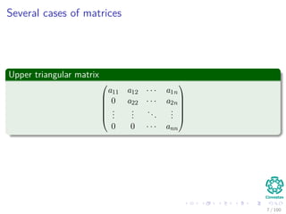
Download as PDF, PPTX


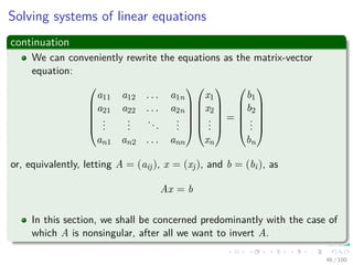
![Complexity and Algorithm
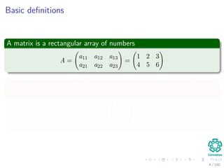
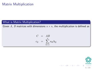
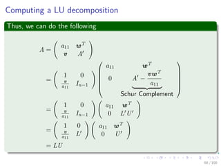
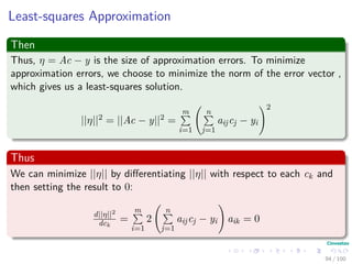
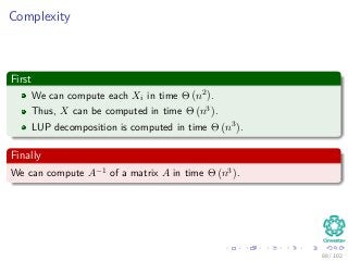
Algorithm: Complexity Θ (n3
)
Square-Matrix-Multiply(A, B)
1 n = A.rows
2 let C be a new matrix n × n
3 for i = 1 to n
4 for j = 1 to n
5 C [i, j] = 0
6 for k = 1 to n
7 C [i, j] = C [i, j] + A [i, j] ∗ B [i, j]
8 return C
12 / 102](https://image.slidesharecdn.com/23matrixalgorithms-151120042533-lva1-app6891/85/23-Matrix-Algorithms-16-320.jpg)

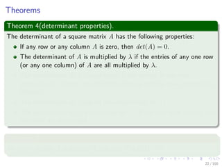
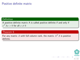
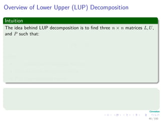
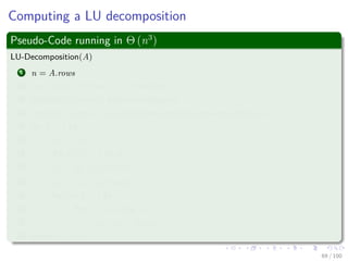
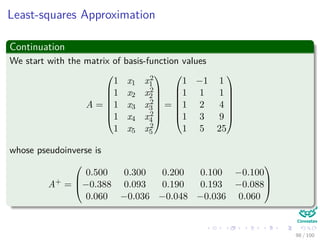
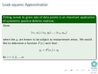
![Determinants
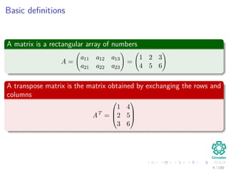
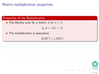
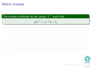
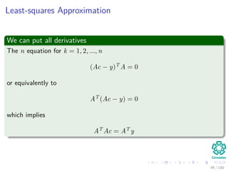
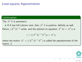
A determinant can be defined recursively as follows
det(A) =
a11 if n = 1
n
j=1
(−1)1+ja1jdet(A[1j]) if n > 1
(1)
Where (−1)i+jdet(A[ij]) is called a cofactor
21 / 102](https://image.slidesharecdn.com/23matrixalgorithms-151120042533-lva1-app6891/85/23-Matrix-Algorithms-31-320.jpg)
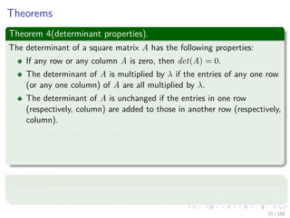
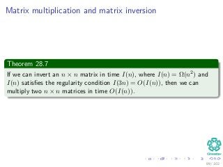
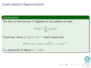
![Determinants
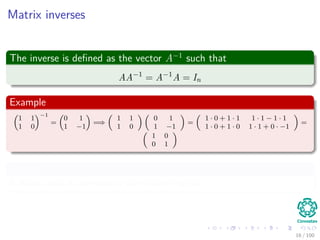
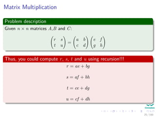
A determinant can be defined recursively as follows
det(A) =
a11 if n = 1
n
j=1
(−1)1+ja1jdet(A[1j]) if n > 1
(1)
Where (−1)i+jdet(A[ij]) is called a cofactor
21 / 102](https://image.slidesharecdn.com/23matrixalgorithms-151120042533-lva1-app6891/85/23-Matrix-Algorithms-32-320.jpg)
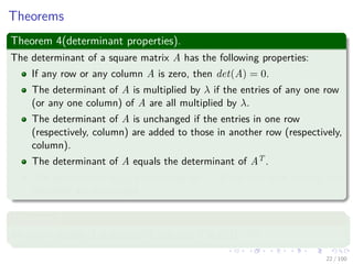

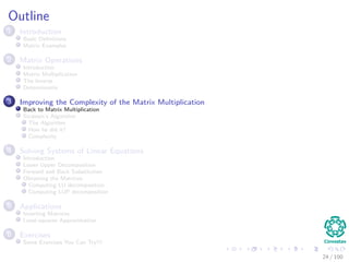


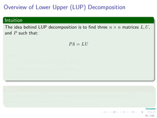
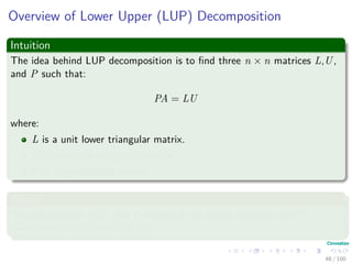
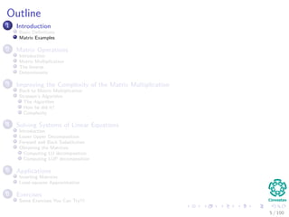
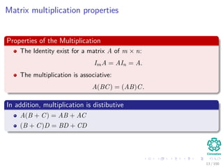
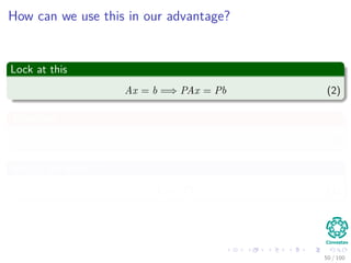
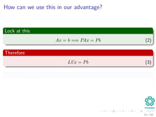
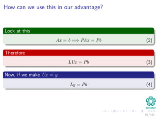
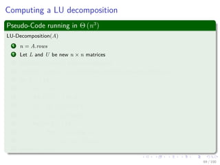
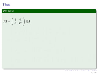
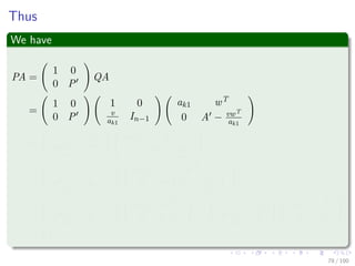
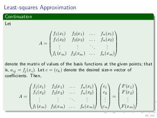
![What is a Permutation Matrix
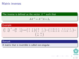
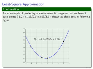
Basically
We represent the permutation P compactly by an array π[1..n]. For
i = 1, 2, ..., n, the entry π[i] indicates that Piπ[i] = 1 and Pij = 0 for
j = π[i].
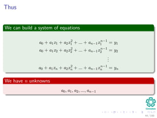
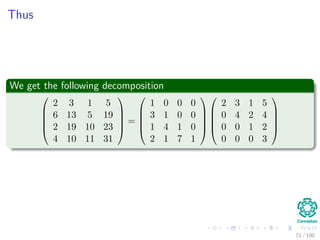
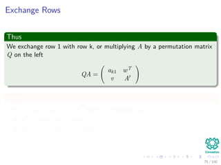
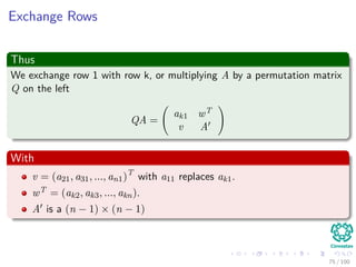
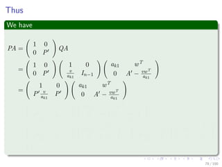
Thus
PA has aπ[i],j in row i and a column j.
Pb has bπ[i] as its ith element.
49 / 102](https://image.slidesharecdn.com/23matrixalgorithms-151120042533-lva1-app6891/85/23-Matrix-Algorithms-107-320.jpg)
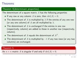
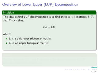
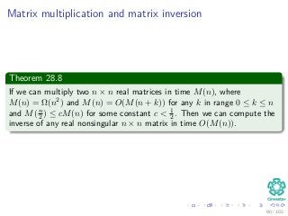
![What is a Permutation Matrix
Basically
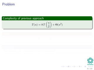
We represent the permutation P compactly by an array π[1..n]. For
i = 1, 2, ..., n, the entry π[i] indicates that Piπ[i] = 1 and Pij = 0 for
j = π[i].
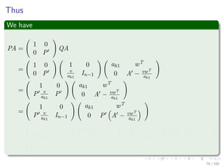
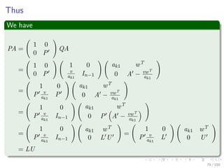
Thus
PA has aπ[i],j in row i and a column j.
Pb has bπ[i] as its ith element.
49 / 102](https://image.slidesharecdn.com/23matrixalgorithms-151120042533-lva1-app6891/85/23-Matrix-Algorithms-108-320.jpg)
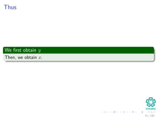
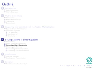
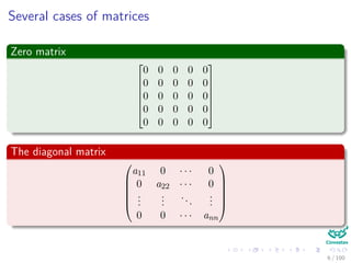
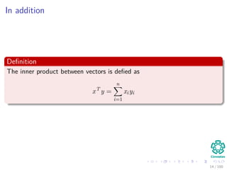
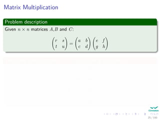
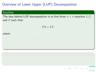
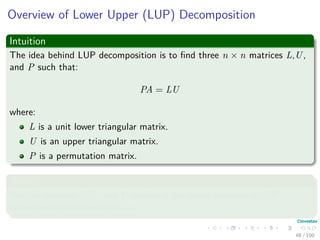
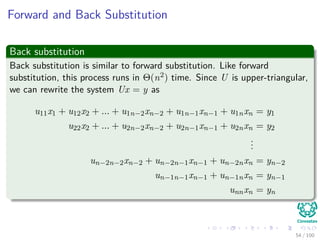
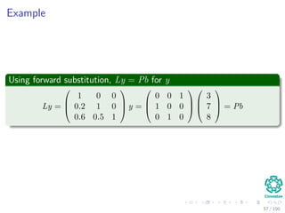
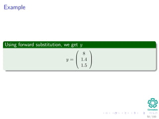
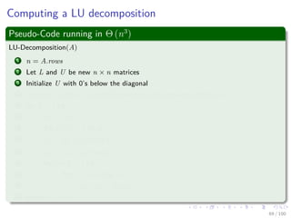
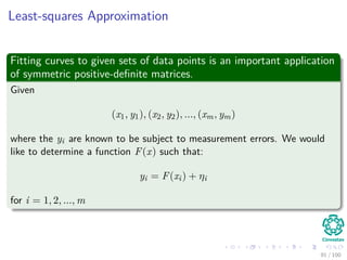
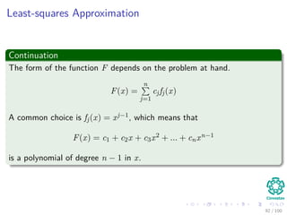
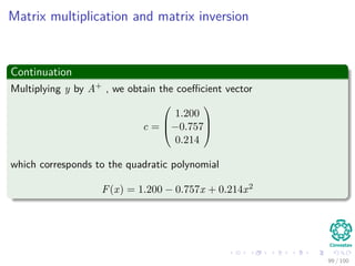
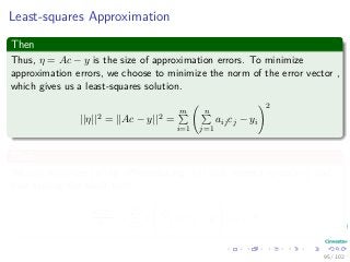
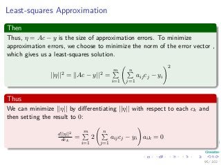
![Forward and Back Substitution
Forward substitution
Forward substitution can solve the lower triangular system Ly = Pb in
Θ(n2) time, given L, P and b.
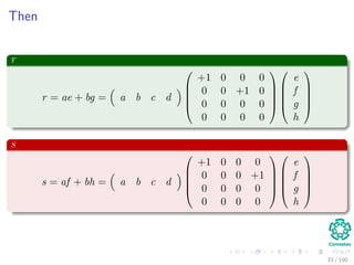
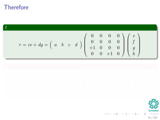
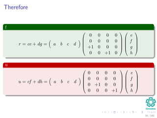
Then
Since L is unit lower triangular, equation Ly = Pb can be rewritten as:
y1 = bπ[1]
l21y1 + y2 = bπ[2]
l31y1 + l32 + y3 = bπ[3]
...
ln1y1 + ln2y2 + ln3y3 + ... + yn = bπ[n]
53 / 102](https://image.slidesharecdn.com/23matrixalgorithms-151120042533-lva1-app6891/85/23-Matrix-Algorithms-114-320.jpg)
![Forward and Back Substitution
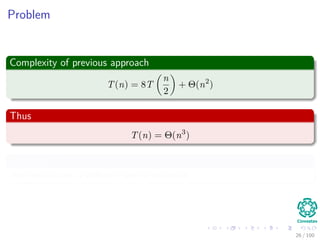
Forward substitution
Forward substitution can solve the lower triangular system Ly = Pb in
Θ(n2) time, given L, P and b.
Then
Since L is unit lower triangular, equation Ly = Pb can be rewritten as:
y1 = bπ[1]
l21y1 + y2 = bπ[2]
l31y1 + l32 + y3 = bπ[3]
...
ln1y1 + ln2y2 + ln3y3 + ... + yn = bπ[n]
53 / 102](https://image.slidesharecdn.com/23matrixalgorithms-151120042533-lva1-app6891/85/23-Matrix-Algorithms-115-320.jpg)
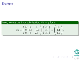
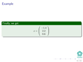
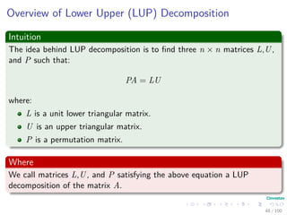
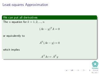
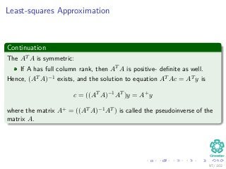
![Forward and Back Substitution
Given P, L, U, and b, the procedure LUP- SOLVE solves for x by
combining forward and back substitution
LUP-SOLVE(L, U, π, b)
1 n = L.rows
2 Let x be a new vector of length n
3 for i = 1 to n
4 yi = bπ[i] − i−1
j=1 lijyj
5 for i = n downto 1
6 xi =
yi−
n
j=i+1
uijxj
uii
7 return x
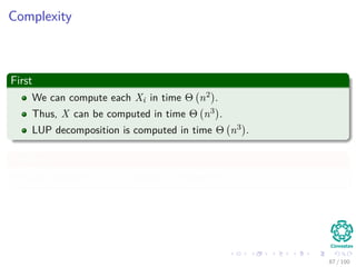
Complexity
The running time is Θ(n2).
61 / 102](https://image.slidesharecdn.com/23matrixalgorithms-151120042533-lva1-app6891/85/23-Matrix-Algorithms-123-320.jpg)
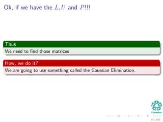
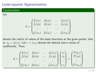
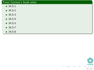
![Forward and Back Substitution
Given P, L, U, and b, the procedure LUP- SOLVE solves for x by
combining forward and back substitution
LUP-SOLVE(L, U, π, b)
1 n = L.rows
2 Let x be a new vector of length n
3 for i = 1 to n
4 yi = bπ[i] − i−1
j=1 lijyj
5 for i = n downto 1
6 xi =
yi−
n
j=i+1
uijxj
uii
7 return x
Complexity
The running time is Θ(n2).
61 / 102](https://image.slidesharecdn.com/23matrixalgorithms-151120042533-lva1-app6891/85/23-Matrix-Algorithms-124-320.jpg)
![Forward and Back Substitution
Given P, L, U, and b, the procedure LUP- SOLVE solves for x by
combining forward and back substitution
LUP-SOLVE(L, U, π, b)
1 n = L.rows
2 Let x be a new vector of length n
3 for i = 1 to n
4 yi = bπ[i] − i−1
j=1 lijyj
5 for i = n downto 1
6 xi =
yi−
n
j=i+1
uijxj
uii
7 return x
Complexity
The running time is Θ(n2).
61 / 102](https://image.slidesharecdn.com/23matrixalgorithms-151120042533-lva1-app6891/85/23-Matrix-Algorithms-125-320.jpg)
![Forward and Back Substitution
Given P, L, U, and b, the procedure LUP- SOLVE solves for x by
combining forward and back substitution
LUP-SOLVE(L, U, π, b)
1 n = L.rows
2 Let x be a new vector of length n
3 for i = 1 to n
4 yi = bπ[i] − i−1
j=1 lijyj
5 for i = n downto 1
6 xi =
yi−
n
j=i+1
uijxj
uii
7 return x
Complexity
The running time is Θ(n2).
61 / 102](https://image.slidesharecdn.com/23matrixalgorithms-151120042533-lva1-app6891/85/23-Matrix-Algorithms-126-320.jpg)
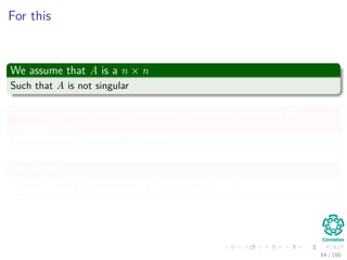
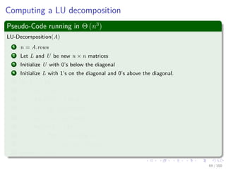
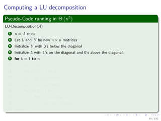
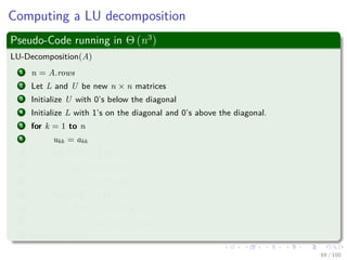
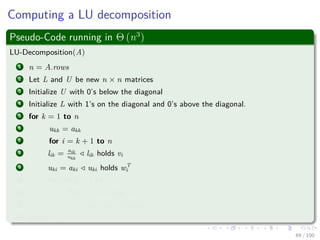
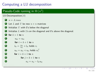
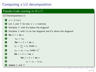
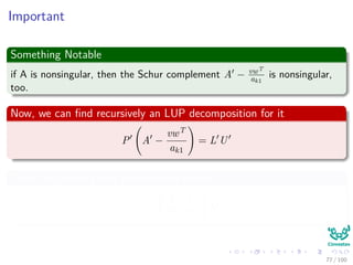
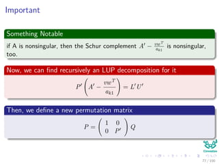

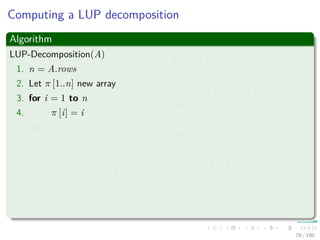
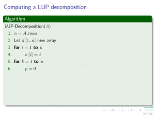
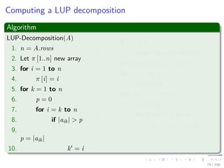
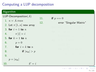
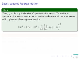
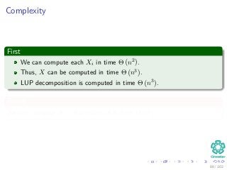
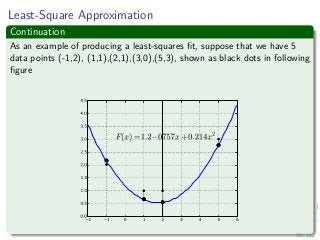
![Computing a LUP decomposition
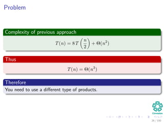
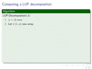
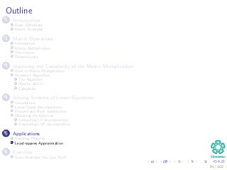
Algorithm
LUP-Decomposition(A)
1. n = A.rows
2. Let π [1..n] new array
3. for i = 1 to n
4. π [i] = i
5. for k = 1 to n
6. p = 0
7. for i = k to n
8. if |aik| > p
9.
p = |aik|
10. k = i
11. if p == 0
12. error “Singular Matrix”
13. Exchange π [k] ←→ π [k ]
14. for i = 1 to n
15. Exchange aki ←→ ak i
16. for i = k + 1 to n
17. aik = aik
akk
18. for j = k + 1 to n
19. aij = aij − aikakj
79 / 102](https://image.slidesharecdn.com/23matrixalgorithms-151120042533-lva1-app6891/85/23-Matrix-Algorithms-180-320.jpg)
![Computing a LUP decomposition
Algorithm
LUP-Decomposition(A)
1. n = A.rows
2. Let π [1..n] new array
3. for i = 1 to n
4. π [i] = i
5. for k = 1 to n
6. p = 0
7. for i = k to n
8. if |aik| > p
9.
p = |aik|
10. k = i
11. if p == 0
12. error “Singular Matrix”
13. Exchange π [k] ←→ π [k ]
14. for i = 1 to n
15. Exchange aki ←→ ak i
16. for i = k + 1 to n
17. aik = aik
akk
18. for j = k + 1 to n
19. aij = aij − aikakj
79 / 102](https://image.slidesharecdn.com/23matrixalgorithms-151120042533-lva1-app6891/85/23-Matrix-Algorithms-181-320.jpg)
![Computing a LUP decomposition
Algorithm
LUP-Decomposition(A)
1. n = A.rows
2. Let π [1..n] new array
3. for i = 1 to n
4. π [i] = i
5. for k = 1 to n
6. p = 0
7. for i = k to n
8. if |aik| > p
9.
p = |aik|
10. k = i
11. if p == 0
12. error “Singular Matrix”
13. Exchange π [k] ←→ π [k ]
14. for i = 1 to n
15. Exchange aki ←→ ak i
16. for i = k + 1 to n
17. aik = aik
akk
18. for j = k + 1 to n
19. aij = aij − aikakj
79 / 102](https://image.slidesharecdn.com/23matrixalgorithms-151120042533-lva1-app6891/85/23-Matrix-Algorithms-182-320.jpg)
![Computing a LUP decomposition
Algorithm
LUP-Decomposition(A)
1. n = A.rows
2. Let π [1..n] new array
3. for i = 1 to n
4. π [i] = i
5. for k = 1 to n
6. p = 0
7. for i = k to n
8. if |aik| > p
9.
p = |aik|
10. k = i
11. if p == 0
12. error “Singular Matrix”
13. Exchange π [k] ←→ π [k ]
14. for i = 1 to n
15. Exchange aki ←→ ak i
16. for i = k + 1 to n
17. aik = aik
akk
18. for j = k + 1 to n
19. aij = aij − aikakj
79 / 102](https://image.slidesharecdn.com/23matrixalgorithms-151120042533-lva1-app6891/85/23-Matrix-Algorithms-183-320.jpg)
![Computing a LUP decomposition
Algorithm
LUP-Decomposition(A)
1. n = A.rows
2. Let π [1..n] new array
3. for i = 1 to n
4. π [i] = i
5. for k = 1 to n
6. p = 0
7. for i = k to n
8. if |aik| > p
9.
p = |aik|
10. k = i
11. if p == 0
12. error “Singular Matrix”
13. Exchange π [k] ←→ π [k ]
14. for i = 1 to n
15. Exchange aki ←→ ak i
16. for i = k + 1 to n
17. aik = aik
akk
18. for j = k + 1 to n
19. aij = aij − aikakj
79 / 102](https://image.slidesharecdn.com/23matrixalgorithms-151120042533-lva1-app6891/85/23-Matrix-Algorithms-184-320.jpg)
![Computing a LUP decomposition
Algorithm
LUP-Decomposition(A)
1. n = A.rows
2. Let π [1..n] new array
3. for i = 1 to n
4. π [i] = i
5. for k = 1 to n
6. p = 0
7. for i = k to n
8. if |aik| > p
9.
p = |aik|
10. k = i
11. if p == 0
12. error “Singular Matrix”
13. Exchange π [k] ←→ π [k ]
14. for i = 1 to n
15. Exchange aki ←→ ak i
16. for i = k + 1 to n
17. aik = aik
akk
18. for j = k + 1 to n
19. aij = aij − aikakj
79 / 102](https://image.slidesharecdn.com/23matrixalgorithms-151120042533-lva1-app6891/85/23-Matrix-Algorithms-185-320.jpg)
![Computing a LUP decomposition
Algorithm
LUP-Decomposition(A)
1. n = A.rows
2. Let π [1..n] new array
3. for i = 1 to n
4. π [i] = i
5. for k = 1 to n
6. p = 0
7. for i = k to n
8. if |aik| > p
9.
p = |aik|
10. k = i
11. if p == 0
12. error “Singular Matrix”
13. Exchange π [k] ←→ π [k ]
14. for i = 1 to n
15. Exchange aki ←→ ak i
16. for i = k + 1 to n
17. aik = aik
akk
18. for j = k + 1 to n
19. aij = aij − aikakj
79 / 102](https://image.slidesharecdn.com/23matrixalgorithms-151120042533-lva1-app6891/85/23-Matrix-Algorithms-186-320.jpg)
![Computing a LUP decomposition
Algorithm
LUP-Decomposition(A)
1. n = A.rows
2. Let π [1..n] new array
3. for i = 1 to n
4. π [i] = i
5. for k = 1 to n
6. p = 0
7. for i = k to n
8. if |aik| > p
9.
p = |aik|
10. k = i
11. if p == 0
12. error “Singular Matrix”
13. Exchange π [k] ←→ π [k ]
14. for i = 1 to n
15. Exchange aki ←→ ak i
16. for i = k + 1 to n
17. aik = aik
akk
18. for j = k + 1 to n
19. aij = aij − aikakj
79 / 102](https://image.slidesharecdn.com/23matrixalgorithms-151120042533-lva1-app6891/85/23-Matrix-Algorithms-187-320.jpg)
![Computing a LUP decomposition
Algorithm
LUP-Decomposition(A)
1. n = A.rows
2. Let π [1..n] new array
3. for i = 1 to n
4. π [i] = i
5. for k = 1 to n
6. p = 0
7. for i = k to n
8. if |aik| > p
9.
p = |aik|
10. k = i
11. if p == 0
12. error “Singular Matrix”
13. Exchange π [k] ←→ π [k ]
14. for i = 1 to n
15. Exchange aki ←→ ak i
16. for i = k + 1 to n
17. aik = aik
akk
18. for j = k + 1 to n
19. aij = aij − aikakj
79 / 102](https://image.slidesharecdn.com/23matrixalgorithms-151120042533-lva1-app6891/85/23-Matrix-Algorithms-188-320.jpg)


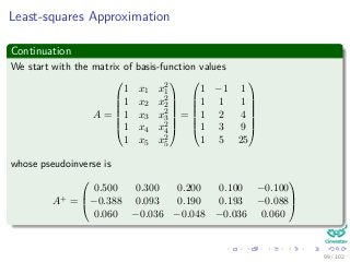
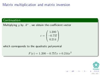
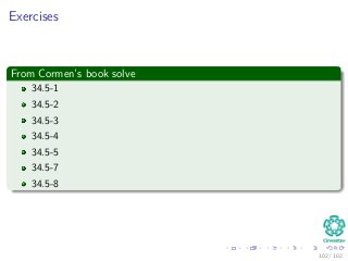

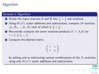
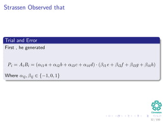
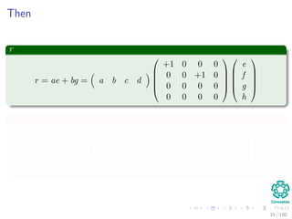
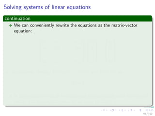
The document provides a comprehensive analysis of matrix algorithms, covering basic definitions, operations, and applications of matrices. It discusses matrix multiplication, Strassen's algorithm, solving systems of linear equations, and properties of determinants and inverses. Additionally, it includes exercises for practical application of the concepts presented.