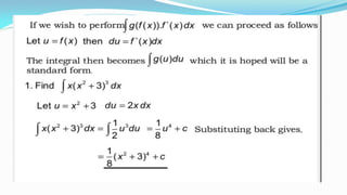
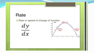
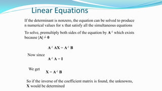
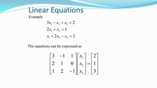
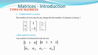
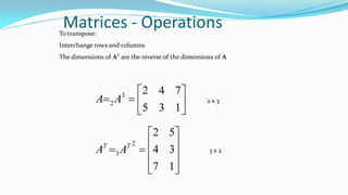
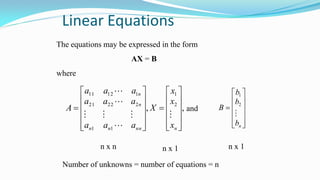
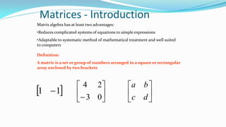
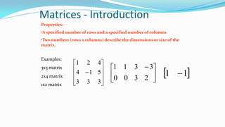
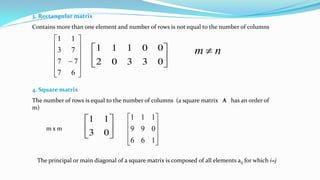
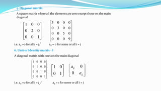
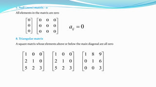
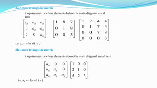
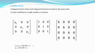
The document provides information about matrices, including: 1) Matrices can reduce complex systems of equations to simple expressions and are well-suited to computers. 2) A matrix is a set of numbers arranged in rows and columns, with specified dimensions. 3) There are several types of matrices including column/row vectors, rectangular, square, diagonal, identity, null, triangular, and scalar matrices. 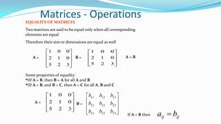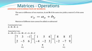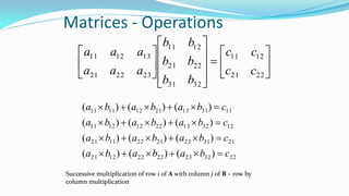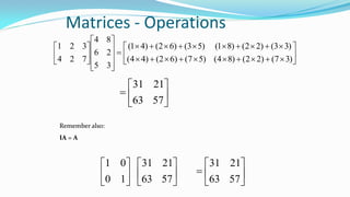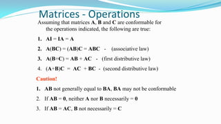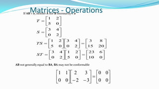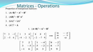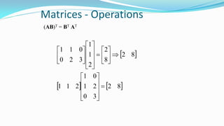4) Matrix operations include addition, subtraction, and multiplication according to specific rules like the distributive property. Not all matrices can be multiplied together.

1. CALCULUS & MATRICES

18. Differential calculus

27. MATRICES

28. Matrices - Introduction
Matrix algebra has at least two advantages:
•Reduces complicated systems of equations to simple expressions
•Adaptable to systematic method of mathematical treatment and well suited
to computers
Definition:
A matrix is a set or group of numbers arranged in a square or rectangular
array enclosed by two brackets
 11  





 03
24






dc
ba

29. Matrices - Introduction
Properties:
•A specified number of rows and a specified number of columns
•Two numbers (rows x columns) describe the dimensions or size of the
matrix.
Examples:
3x3 matrix
2x4 matrix
1x2 matrix











333
514
421





 
2
3
3
3
0
1
0
1
 11 

30. Matrices - Introduction
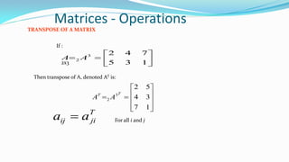
A matrix is denoted by a bold capital letter and the elements within the matrix
are denoted by lower case letters
e.g. matrix [A] with elements aij














mnijmm
nij
inij
aaaa
aaaa
aaaa
21
22221
1211
...
...

i goes from 1 to m
j goes from 1 to n
Amxn=
mAn

31. Matrices - Introduction
TYPES OF MATRICES
1. Column matrix or vector:
The number of rows may be any integer but the number of columns is always 1










2
4
1






3
1












1
21
11
ma
a
a

2. Row matrix or vector
Any number of columns but only one row
 611  2530
 naaaa 1131211 

32. 3. Rectangular matrix
Contains more than one element and number of rows is not equal to the number of columns













67
77
73
11






03302
00111 nm 
4. Square matrix
The number of rows is equal to the number of columns (a square matrix A has an order of
m)
m x m 





03
11










166
099
111
The principal or main diagonal of a square matrix is composed of all elements aij for which i=j

33. 5. Diagonal matrix
A square matrix where all the elements are zero except those on the main
diagonal










100
020
001












9000
0500
0030
0003
i.e. aij =0 for all i = j aij = 0 for some or all i = j
6. Unit or Identity matrix - I
A diagonal matrix with ones on the main diagonal












1000
0100
0010
0001






10
01






ij
ij
a
a
0
0
i.e. aij =0 for all i = j aij = 1 for some or all i = j

34. 7. Null (zero) matrix - 0
All elements in the matrix are zero










0
0
0










000
000
000
0ija
8. Triangular matrix
A square matrix whose elements above or below the main diagonal are all zero










325
012
001










325
012
001










300
610
981

35. 8a. Upper triangular matrix
A square matrix whose elements below the main diagonal are all
zero
i.e. aij = 0 for all i > j










300
810
781












3000
8700
4710
4471










ij
ijij
ijijij
a
aa
aaa
00
0
8b. Lower triangular matrix
A square matrix whose elements above the main diagonal are all zero










ijijij
ijij
ij
aaa
aa
a
0
00










325
012
001
i.e. aij = 0 for all i < j

36. 9. Scalar matrix
A diagonal matrix whose main diagonal elements are equal to the same scalar
A scalar is defined as a single number or constant










100
010
001












6000
0600
0060
0006
i.e. aij = 0 for all i = j
aij = a for all i = j










ij
ij
ij
a
a
a
00
00
00

37. Matrix Operations

38. Matrices - Operations
EQUALITY OF MATRICES
Two matrices are said to be equal only when all corresponding
elements are equal
Therefore their size or dimensions are equal as well










325
012
001










325
012
001
A = B = A = B
Some properties of equality:
•IIf A = B, then B = A for all A and B
•IIf A = B, and B = C, then A = C for all A, B and C










325
012
001










333231
232221
131211
bbb
bbb
bbb
A = B =
If A = B then
ijij ba 

39. Matrices - OperationsADDITION AND SUBTRACTION OF MATRICES
The sum or difference of two matrices, A and B of the same size yields a matrix C of the same
size
ijijij bac 
Matrices of different sizes cannot be added or subtracted
Commutative Law:
A + B = B + A
Associative Law:
A + (B + C) = (A + B) + C = A + B + C






















972
588
324
651
652
137
A
2x3
B
2x3
C
2x3

40. Matrices - Operations























2221
1211
3231
2221
1211
232221
131211
cc
cc
bb
bb
bb
aaa
aaa
22322322221221
21312321221121
12321322121211
11311321121111
)()()(
)()()(
)()()(
)()()(
cbababa
cbababa
cbababa
cbababa




Successive multiplication of row i of A with column j of B – row by
column multiplication

41. Matrices - Operations

























)37()22()84()57()62()44(
)33()22()81()53()62()41(
35
26
84
724
321







5763
2131
Remember also:
IA = A






10
01






5763
2131







5763
2131

42. Matrices - Operations
Assuming that matrices A, B and C are conformable for
the operations indicated, the following are true:
1. AI = IA = A
2. A(BC) = (AB)C = ABC - (associative law)
3. A(B+C) = AB + AC - (first distributive law)
4. (A+B)C = AC + BC - (second distributive law)
Caution!
1. AB not generally equal to BA, BA may not be conformable
2. If AB = 0, neither A nor B necessarily = 0
3. If AB = AC, B not necessarily = C

43. Matrices - Operations
AB not generally equal to BA, BA may not be conformable




















































010
623
05
21
20
43
2015
83
20
43
05
21
20
43
05
21
ST
TS
S
T
If AB = 0, neither A nor B necessarily = 0


















00
00
32
32
00
11

44. Matrices - Operations
TRANSPOSE OF A MATRIX
If :







135
7423
2 AA
2x3











17
34
52
3
2
TT
AA
Then transpose of A, denoted AT is:
T
jiij aa  For all i and j

45. Matrices - OperationsTo transpose:
Interchange rows and columns
The dimensions of AT are the reverse of the dimensions of A







135
7423
2 AA











17
34
52
2
3
TT
AA
2 x 3
3 x 2

46. Matrices - OperationsProperties of transposed matrices:
1. (A+B)T = AT + BT
2. (AB)T = BT AT
3. (kA)T = kAT
4. (AT)T = A
1. (A+B)T = AT + BT






















972
588
324
651
652
137












95
78
28






































95
78
28
36
25
41
61
53
27

47. Matrices - Operations
(AB)T = BT AT
 
   82
30
21
01
211
82
8
2
2
1
1
320
011



































48. Matrices - Operations
SYMMETRIC MATRICES
A Square matrix is symmetric if it is equal to its
transpose:
A = AT














db
ba
A
db
ba
A
T

49. Matrices - Operations
When the original matrix is square, transposition does not
affect the elements of the main diagonal














db
ca
A
dc
ba
A
T
The identity matrix, I, a diagonal matrix D, and a scalar matrix, K,
are equal to their transpose since the diagonal is unaffected.

50. Matrices - Operations
INVERSE OF A MATRIX
Consider a scalar k. The inverse is the reciprocal or division of 1
by the scalar.
Example:
k=7 the inverse of k or k-1 = 1/k = 1/7
Division of matrices is not defined since there may be AB = AC
while B = C
Instead matrix inversion is used.
The inverse of a square matrix, A, if it exists, is the unique matrix
A-1 where:
AA-1 = A-1 A = I

51. Matrices - Operations
Example:

















32
11
12
13
1
2
2
A
AA








































10
01
32
11
12
13
10
01
12
13
32
11
Because:

52. Matrices - Operations
ADJOINT MATRICES
A cofactor matrix C of a matrix A is the square matrix of the same
order as A in which each element aij is replaced by its cofactor cij .
Example:








43
21
A








12
34
C
If
The cofactor C of A is

53. Matrices - Operations
The adjoint matrix of A, denoted by adj A, is the transpose of its cofactor matrix
T
CadjA 
It can be shown that:
A(adj A) = (adjA) A = |A| I
Example:





 










13
24
10)3)(2()4)(1(
43
21
T
CadjA
A
A
IadjAA 10
100
010
13
24
43
21
)( 










 








IAadjA 10
100
010
43
21
13
24
)( 
















 


54. Matrices - OperationsUSING THE ADJOINT MATRIX IN MATRIX INVERSION
A
adjA
A 1
Since
AA-1 = A-1 A = I
and
A(adj A) = (adjA) A = |A| I
then
Example






 43
21
A =





 





 

1.03.0
2.04.0
13
24
10
11
A
AA-1 = A-1 A = I
IAA
IAA

















 












 










10
01
43
21
1.03.0
2.04.0
10
01
1.03.0
2.04.0
43
21
1
1
To check

55. Simple 2 x 2 case
So that for a 2 x 2 matrix the inverse can be constructed
in a simple fashion as





















 ac
bd
A
A
a
A
c
A
b
A
d
1
•Exchange elements of main diagonal
•Change sign in elements off main diagonal
•Divide resulting matrix by the determinant







zy
xw
A 1

56. Simple 2 x 2 case
Example

























2.04.0
3.01.0
24
31
10
1
14
32
1
A
A
Check inverse
A-1 A=I
I




















10
01
14
32
24
31
10
1

57. Linear Equations

58. Linear EquationsLinear equations are common and important for survey
problems
Matrices can be used to express these linear equations and
aid in the computation of unknown values
Example
n equations in n unknowns, the aij are numerical coefficients,
the bi are constants and the xj are unknowns
nnnnnn
nn
nn
bxaxaxa
bxaxaxa
bxaxaxa







2211
22222121
11212111

59. Linear Equations
The equations may be expressed in the form
AX = B
where
,, 2
1
11
22221
11211


























nnnnn
n
n
x
x
x
X
aaa
aaa
aaa
A






and













nb
b
b
B

2
1
n x n n x 1 n x 1
Number of unknowns = number of equations = n

60. Linear Equations
If the determinant is nonzero, the equation can be solved to produce
n numerical values for x that satisfy all the simultaneous equations
To solve, premultiply both sides of the equation by A-1 which exists
because |A| = 0
A-1 AX = A-1 B
Now since
A-1 A = I
We get
X = A-1 B
So if the inverse of the coefficient matrix is found, the unknowns,
X would be determined

61. Linear Equations
Example
32
12
23
321
21
321



xxx
xx
xxx
The equations can be expressed as

































3
1
2
121
012
113
3
2
1
x
x
x