This document provides an introduction to machine learning concepts including loss functions, empirical risk, and two basic methods of learning - least squared error and nearest neighborhood. It describes how machine learning aims to find an optimal function that minimizes empirical risk under a given loss function. Least squared error learning is discussed as minimizing the squared differences between predictions and labels. Nearest neighborhood is also introduced as an alternative method. The document serves as a high-level overview of fundamental machine learning principles.

1. Introduction to Machine Learning
Notes
A Basic Introduction to Learning
Andres Mendez-Vazquez
June 4, 2018
1

2. Cinvestav Guadalajara
Contents
1 Introduction 3
2 Loss Functions and Empirical Risk 4
2.1 Empirical Risk as Error Minimization . . . . . . . . . . . . . . . 4
2.2 Example of Risk Minimization, Least Squared Error . . . . . . . 6
3 Two Methods of Learning 7
3.1 Least Squared Error . . . . . . . . . . . . . . . . . . . . . . . . . 8
3.2 Nearest Neighborhood . . . . . . . . . . . . . . . . . . . . . . . . 10
3.3 Machine Learning Methods as combination and improvements of
LSE and k-NN . . . . . . . . . . . . . . . . . . . . . . . . . . . . 11
4 Supervised Learning as Function Approximation 12
4.1 Regression as Controlled Overfitting . . . . . . . . . . . . . . . . 12
4.2 Extreme Fitting, Bias-Variance Problem . . . . . . . . . . . . . . 14
4.2.1 “Extreme” Cases of Fitting . . . . . . . . . . . . . . . . . 16
5 Some Classes of Estimators 18
5.1 Roughness Penalty . . . . . . . . . . . . . . . . . . . . . . . . . . 18
5.2 Kernel Methods and Local Regression . . . . . . . . . . . . . . . 19
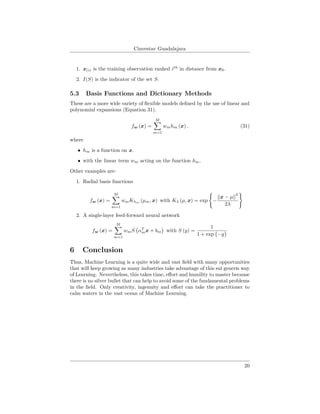
5.3 Basis Functions and Dictionary Methods . . . . . . . . . . . . . . 20
6 Conclusion 20
List of Figures
1 Mapping from the input space into the output space with two
classes . . . . . . . . . . . . . . . . . . . . . . . . . . . . . . . . . 3
2 A Hyperplane splitting the space in . . . . . . . . . . . . . . . . 4
3 The positive subspace R1 and the negative subspace R2 . . . . 5
4 as the difference = y − g (x, w) . . . . . . . . . . . . . . . . . 9
5 Decision Boundary x|wT
x = (l1+l2)/2 . . . . . . . . . . . . . . 10
6 Mahalanobis as a distance measuring the maximum change in
each feature. . . . . . . . . . . . . . . . . . . . . . . . . . . . . . 11
7 The Decision Boundary k = 5 and k = 1. Here k=1 correspond
to a Voronoi diagram [1]. . . . . . . . . . . . . . . . . . . . . . . 11
8 The data and the random observations. . . . . . . . . . . . . . . 13
9 The function used to estimate the output y is highly biased given
the mapping. . . . . . . . . . . . . . . . . . . . . . . . . . . . . . 16
10 The high variance case of fitting . . . . . . . . . . . . . . . . . . 17
11 The cubic smooth spline . . . . . . . . . . . . . . . . . . . . . . . 18
12 Two types of Kernels . . . . . . . . . . . . . . . . . . . . . . . . . 19
2

3. Cinvestav Guadalajara
Figure 1: Mapping from the input space into the output space with two classes
1 Introduction
As in any other field of Science, it is necessary to obtain a basic understanding of
the subject before getting into the main matter of the subject. In our particular
case, the concept of “Learning” in Machine Learning [2, 3, 4, 5]. As we will see
through our study of Machine Learning, we could give the following definition
of “Learning.”[6]
Definition 1.1. Given that the information of an object has been summarized
by d features comprised as a feature vector x ∈ Rd
, and each of these objects
has been labeled by elements in a set {yi ∈ R}. This allows to split the set of
object into a series classes, as for example yi ∈ {−1, 1}. Then, for example,
the process of learning is the generation of a mapping f : Rd
→ {yi} (Figure
1) such that the squared error estimation of the class label of a new sample is
minimized (Equation 1).
min
f
EX,Y f (x) − y
2
|x ∈ X ⊆ Rd
, y ∈ Y ⊆ R (1)
Although this task looks quite simple, actually it can be quite complex!
Therefore, a good starting point to this endeavors is to use our analytic ge-
ometry [7] from high school to try to obtain such mapping. Thus, if we use a
geometric approach, and assuming two linearly separable classes, we could start
by splitting the samples into two set of elements,
C1 = xi ∈ Rd
|yi = 0
C2 = xi ∈ Rd
|yi = 1
Then, we could try to obtain a geometric function allowing to split the space
of inputs into two classes. For example, we could use (Figure 2) .
3

4. Cinvestav Guadalajara
Figure 2: A Hyperplane splitting the space in
f (x) = wT
x + w0 (2)
Question, How does this function split the space in R3
? The answer comes from
the equation (Equation 3).
wT
x = w x cos θ (3)
Basically, θ represents the angle between vectors w and x. Thus, we have
the following rule:
1. If 0 ≤ θ ≤ 90 then wT
x ≥ 0
2. If θ > 90, then wT
x < 0
Therefore, w defines a positive subspace and a negative subspace (Figure 3)
given the direction defined by the vector.
A question arises naturally, from this first approach, How do you obtain such
function? We will see a first approach for this in the following section.
2 Loss Functions and Empirical Risk
2.1 Empirical Risk as Error Minimization
The first thing that you need to think about, while trying to obtain an estimation
mapping between the input space X and the output space Y, is our decision
about how to relate the two variables, the vectors x ∈ Rd
and the outputs y ∈ R.
Example 2.1. We could try to relate the variations in prices at supermarkets
with thSkycatch e variations in salary by assuming a growing economy [8]. Given
such scenario, you could think a linear relation like (Equation 4).
4

5. Cinvestav Guadalajara
Figure 3: The positive subspace R1 and the negative subspace R2
∆P = w0 + w1∆S + (4)
with ∆P and ∆S are the price and salary variations, w0 and w1 are unknown
coefficients and ∼ N(0, σ2
).
This example depicts one of the classic models in the literature, the linear
models where a random source of noise is used to model the variability on the yi
being observed. Now, given the previous linear random relation, anybody will
start to wonder how to minimize the noise or error (Equation 5),
= ∆P − (w0 + w1∆S) . (5)
Given that we want to minimize such error, we require to compose the pre-
vious functions with an specific one to obtain the desired results. For this, we
introduce the idea of statistical risk as a functional that evaluates the expected
value of a function that describe a measure of loss.
Definition 2.2. (Principle of Empirical Risk) [9] Given a sequence of data sam-
ples, x1, x2, ..., xN sampled iid from a distribution P (x|Θ), and an hypothesis
function h : X → Y that allows to map the samples xi into a particular output
yi. A measure of the risk of missing the estimation, h (x), is found by using
a function, called loss function, measuring the difference between the desired
output yi and the estimation h (xi). Thus, the Empirical Risk is defined as
the expected value of the loss function based in the joint distribution P (x, y)
(Equation 6).
R (h) = EX,Y [ (h (x) , y)] =
X,Y
(h (x) , y) p (x, y) dxdy (6)
Examples of such loss functions are (Equation 7):
5

6. Cinvestav Guadalajara
h (w0, w1) = [∆P − (w0 + w1∆S)]
2
(Least Squared Error),
h (w0, w1) = |∆P − (w0 + w1∆S)| (Absolute Difference), (7)
h (w0, w1) =
1
1 + exp {− (w0 + w1∆S)}
(Sigmoidal).
After looking at such functions loss functions, one could ask, Is there a way
to obtain the optimal function h that minimizes their Empirical Risks? Is there
a way to find the optimal loss function for a given data set {(xi, yi)}? These
simple questions have driven the Machine Learning endeavor for the last 60
years.
2.2 Example of Risk Minimization, Least Squared Error
To exemplify the idea of minimizing the Risk Function [3], let us to select a
convenient loss function:
L (y, f (x)) = (y − f (x))
2
(Least Squared Error) (8)
Here, we select a functional relation between the outputs y s and inputs x s:
Ynoisy (x) = f (y) + with ∼ N (0, 1) (9)
Then, we have the following Risk functional [9, 3]:
R (f) = E (Y − f (X))
2
=
X Y
[y − f (x)]
2
pxy (x, y) dxdy
Now, we can condition the probability density function with respect to X:
p (X, Y ) = p (Y |X) p (X)
Therefore, we have
X Y
[y − f (x)]
2
pxy (x, y) dxdy =
X Y
[y − f (x)]
2
py|x (y|x) px (x) dxdy
=
X Y
[y − f (x)]
2
py|x (y|x) dy dx
= EX
Y
[y − f (x)]
2
py|x (y|x) dy
= EXEY |X (Y − f (X))
2
|X
Thus, if we fix X = x, we have that the Risk functional is with respect to
such x :
R (f)X=x = EY |X=x (Y − f (x))
2
|X = x
This function can be optimized by realizing that
6

7. Cinvestav Guadalajara
EY |X=x (Y − f (x))
2
|X = x = EY |X=x Y − Y
2
|X = x + ... =
EY |X=x Y − f (x)
2
|X = x + ...
2 Y − f (x) EY |X=x Y − Y |X = x
Then, you notice that
EY |X=x Y − Y |X = x = EY |X=x [Y ] − EY |X=x
1
N
N
i=1
Yi
= µY −
1
N
N
i=1
EY |X=x [Yi]
= µY −
NµY
N
= 0
Thus, we have
EY |X=x (Y − f (x))
2
|X = x = EY |X=x Y − Y
2
|X = x + ...
EY |X=x Y − f (x)
2
|X = x
Therefore, if we choose
f (X) = Y ≈ EY [Y |X = x]
Thus, we finish with
EY |X=x (Y − f (x))
2
|X = x = EY |X=x (Y − EY [Y |X = x])
2
|X = x = σ2
Y = 1,
the variance of Y ∼ N (EY [Y |X = x] , 1) when choosing f (X) = EY [Y |X = x]
given ∼ N (0, 1). This means that the optimal estimator is the conditional
mean for a point X = x, when measured by the expected squared error.
3 Two Methods of Learning
Therefore, given the Empirical Risk, we can think on the process of “learning”
as the process of finding an optimal function h that minimizes such risk under
an specific loss function/learning model. Clearly, this process does not take in
account an important issue in the human process of learning:
• How a human being uses few samples to generalize a concept?
For example, once a child learns the concept of “cat,” she/he will be able to rec-
ognize almost every cat over the planet. Although, the concept of generalization
exists in Machine Learning as part of the Bias-Variance problem [2, 3, 5], little
progress has been done toward a sparse inductive generalization. Nevertheless,
7

8. Cinvestav Guadalajara
there have been claims in the Deep Neural Network field of new generalization
powers [10] by those devices. However, those powers require massive amounts
of data, unlikely as the human child learning something as not so simple as a
“cat.”
After the previous digression, it is time to go back to our main topic, the
process of “Learning” in Machine Learning. For this, we will take a look at two
different methods of learning that could be seen as the extremes of a line where
the Machine Learning methods live.
3.1 Least Squared Error
Here, we have the following situation about the data samples of a given classi-
fication problem:
• A sequence of samples with their respective labels, {(x1, y1) , (x2, y2) , ..., (xN , yN )}
• Here, each xi ∈ Rd
and yi ∈ R with i = 1, 2, ..., N.
Then, it is possible to use the squared loss function, under a function g estimat-
ing the outputs yis:
(g (x) , y) = (g (x) − y)
2
(10)
Thus, we have:
R (g) =
X,Y
(g (x) , y) p (x, y) dxdy =
N
i=1
(g (xi) − yi)
2
p (xi, yi) . (11)
Now, if assume two classes at the data i.e. yi ∈ {l1, l2|li ∈ R} such that
|Cl1 | = |Cl2 |
p (xi, yi) =
|Cl1
|
N
≈
1
2
if xi ∈ Cl1
,
p (xi, yi) =
|Cl2
|
N
≈
1
2
if xi ∈ Cl2
.
Therefore,
R (g) =
N
i=1
(g (xi) − yi)
2
p (xi, yi) =
1
2
N
i=1
(g (xi) − yi)
2
.
Now, in the specific case of a linear model like g (x, w) = w0 + wT
x, it is
possible to relate the output through a random error :
y = g (x, w) + , (12)
thus, the error can be seen graphically as (Figure 4).
Here, a simplifying assumption is that the error comes from a Gaussian
Distribution with mean 0 and variance σ2
, N 0, σ2
. Therefore, the Risk
Functional can be rewritten as
8

9. Cinvestav Guadalajara
Figure 4: as the difference = y − g (x, w)
E (w) =
1
2
N
i=1
2
=
1
2
N
i=1
w0 + wT
x − yi
2
(13)
Finally, using our Linear Algebra knowledge, we can rewrite this Risk Func-
tional as
E (w) = (y − Xw)
T
(y − Xw) (14)
with
X =








1 (x1)1 · · · (x1)j · · · (x1)d
...
...
...
1 (xi)1 (xi)j (xi)d
...
...
...
1 (xN )1 · · · (xN )j · · · (xN )d








, y =





y1
y2
...
yN





(15)
The final solution, the estimation w, is
w = XT
X
−1
XT
y (16)
A question arises, how do we use this w to obtain the labels of our classes?
We define a threshold saying (l1+l2)/2 and we define the rule of classification
GLSE (x) =
Class 1 if wT
x > (l1+l2)/2
Class2 if wT
x ≤ (l1+l2)/2
Thus, we have that the hyperplane defined by w is a decision boundary
that allows to split the space Rd+1
into two classes (Figure 5). As you can see,
decision boundary is splitting the space into two sub-planes where, as you can
see, you can still have miss-classifications when estimating labels for the data
samples.
This represent one of the most popular models in Statistics [11]. Addition-
ally, it is one of the basic models of Learning in Machine Learning.
9

10. Cinvestav Guadalajara
Figure 5: Decision Boundary x|wT
x = (l1+l2)/2
3.2 Nearest Neighborhood
The other basic model in Machine Learning is the well known k-Nearest Neigh-
bor (k-NN) model. This model can be though as an answer to the problem
of increasing complexity of estimation of h, when the number of dimensions
increases beyond a certain level. The rule of classification is quite simple:
y (x) =
1
k xi∈Nk(x)
yi
where NK (x) is the neighborhood of x defined by the k closest point xi
1
. Here,
an important questions is: What is the metric used to establish the concept of
“near”? For example, we have the concept of near in documents by using the
metric:
J (D1, D2) =
|D1 ∩ D2|
|D1| + |D2| − |D1 ∩ D2|
(Jaccard Index)
when Di is the vector that registers if a word appears or not in the document.
Another example comes from the idea of using the sample mean and the sample
covariance of Data Matrix (Equation 15).
X =
1
N
N
i=1
xi1 xi2 · · · xip
T
(Sample Mean),
CX =
1
N − 1
X − X
T
X − X (Sample Covarance).
This allows to define the Mahalanobis Distance (Figure 6), and as in the
previous Least Squared Error, we can define a new rule of classification based
1Here, an efficient data structure to find the elements of NK (x) are know as the K − d
trees [12]. This is necessary, if we want to have efficient Learning algorithms for Large Data
sets.
10

11. Cinvestav Guadalajara
Figure 6: Mahalanobis as a distance measuring the maximum change in each
feature.
Figure 7: The Decision Boundary k = 5 and k = 1. Here k=1 correspond to a
Voronoi diagram [1].
on:
Gk-NN (x) =
Class 1 if 1
k xi∈Nk(x) yi > (l1+l2)/2
Class 2 if 1
k xi∈Nk(x) yi ≤ (l1+l2)/2
,
where different values for k can produce different boundary decisions (Figure
7).
3.3 Machine Learning Methods as combination and im-
provements of LSE and k-NN
Something of great interest, as people looking for Patterns in the mathematical
structures, mathematical models and data, is the realization that many methods
in Machine Learning are related in many ways. In this regards, Hastie et. al
[3] have identified two main algorithms for Learning, the Least Squared Error
(Section 3.1) and k-Nearest Neighbor (Section 3.2), that can bee seen as the
two main basis for the algorithms in Machine Learning.
11

12. Cinvestav Guadalajara
For example, in the case of Support Vector Machines [13], when looking at
its dual solution by Vapnik [4]:
Q (α) =
N
i=1
αi −
1
2
N
i=1
N
j=1
αiαjdidjxT
j xi (17)
It is know that the elements αi are different from zero when its associated vector
is a support vector. Using an arbitrary kernel in (Equation 17), it is possible to
rewrite the equation as:
N
i=1
αi −
1
2
N
i=1
N
j=1
αiαjdidjK (xj, xi) . (18)
Thus, if we assume
(αi, αj, di, dj) = I (αi > t, αj > t) sign (didj) ,
and p = 1, we have
N
i=1

αi −
1
2
N
j=1
(αi, αj, di, dj) K (xj, xi)


p
(19)
Which looks like a Linear Regression with αi as the desired output and
f (xi) =
1
2
N
j=1
(αi, αj, di, dj) K (xj, xi)
as the estimator of sample xi based on their projections by K (xj, ∗).
This is one example of many where algorithms in Machine Learning can be
seen as an extension of LSE or k-NN. These could be seen as a little bit lim-
ited, but it is useful when trying to analyze and categorize a Machine Learning
Algorithm when doing model selection [14].
4 Supervised Learning as Function Approxima-
tion
4.1 Regression as Controlled Overfitting
In an exemplifying case, we observe a real-valued input variable x ∈ R, and we
are looking to predict the value of a real valued variable y ∈ R. Thus, we have
a vector of tuples:
D = {(xi, yi) |i = 1, 2, ..., N} (20)
for the N samples with their respective outputs. For example, we have the
function:
12

13. Cinvestav Guadalajara
Figure 8: The data and the random observations.
g (x) = f (x) + α (21)
with ∼ U (0, 1), α > 0, f (x) = sin {x} and x ∈ R (Figure 8).
Thus, our goal is to exploit this training set to reduce the noise introduced
by the system and our observations (Kalman [15]). Basically, we want make
predictions of the value y = g (x) given a new value x. For this is possible to
propose the following polynomial:
y = g (x, w) =
d
i=0
wixi
,
which can be seen as a generation of new features in a polynomial way (Poly-
nomial Kernels [13]). These functions are linear at the parameter w and are
called linear models. The question, How do we fit the model to our data? Here,
we can use the sum of squared errors:
R (w) =
1
2
N
i=1
[g (xi, w) − yi]
2
(22)
Later in the section of linear models, we will look at ways to get the the canonical
solution (Equation 16) for the problem. However, in general, the goal is to to
obtain a useful approximation (fitting) to g(x, w) for all x in some region of Rd
, given the representations in D. This is an advantage because we can use all
the tools generated in the last 200 years for function approximation. Making
the task of Approximation/Supervised Learning as Controlled Overfitting
where in each model a series of parameters are approximated to obtain the
desired fitting.
Examples of different approximations that relate the labels and samples in
D are:
13

14. Cinvestav Guadalajara
1. The linear model f (x) = xT
w with θ = w.
2. The linear basis expansion
fθ (x) =
K
k=1
hk (x) θk
with hk (x) = x2
1 or hk (x) = 1
1+exp{−xT θk}
and many other ones.
3. The residual sum of squared errors
RSS (fw, x0) =
N
i=1
Kλ (xi, x0) (yi − fw (xi))
2
Although these are some examples that are quite important in the process of
approximation, one should ask the following question, When do we have fittings
that are not good at all for the data space? In the following section, we try to
answer this question.
4.2 Extreme Fitting, Bias-Variance Problem
For the following development [16, 17], we will take a look at the underlying
probability of the samples x s by having the following assumptions:
1. There is an underlying distribution for the data xi ∼ p (x|Θ) [18]. Here,
the notation p (x|Θ) represent the random dependencies of the samples of
the underlaying distribution p which is parametrized by Θ.
2. Some Learning Algorithm has been able to find an estimation function
g (x|D) where the notation |D represents the dependency of the function
g to the training data D.
3. As in the Least Squared Error, we have seen that the optimal solution for
the regression ED [y|x] where the subscript D means that the expected
value depends on the distribution P (X, Y ).
4. The noise added by the mapping y = g (x) + has a distribution ∼
N 0, σ2
.
Then, from our probability theory the V ar (X) = E (X − µ)
2
which can be
used to measure the error (Equation 23) of the function g (x|D) with respect to
such expected label of a given sample, E [y|x].
V arD (g (x|D)) = ED g (x|D) − ED -NN [y|x]
2
(23)
Clearly as part of measuring the error, we can use the expected value of the
trained function/machine g (x|D) (Equation 24).
14

15. Cinvestav Guadalajara
ED [g (x|D)] (24)
the expected output of the machine. Thus, by using a little of algebra, we can
rewrite (Equation 23) as
V arD (g (x|D)) = ED (g (x|D) − ED [y|x])
2
= ED (g (x|D) − E [g (x|D)] + E [g (x|D)] − ED [y|x])
2
= ED (g (x|D) − ED [g (x|D)])
2
+ ...
...2 (g (x|D) − ED [g (x|D)]) (ED [g (x|D)] − ED [y|x]) + ...
... (ED [g (x|D)] − ED [y|x])
2
.
We can split the terms using the linearity of the expected value:
V arD (g (x|D)) = ED (g (x|D) − ED [g (x|D)])
2
+ ...
...2ED [(g (x|D) − ED [g (x|D)]) (ED [g (x|D)] − ED [y|x])] + ...
...ED (ED [g (x|D)] − ED [y|x])
2
.
The central term is one of interest
ED [(g (x|D) − ED [g (x|D)]) (ED [g (x|D)] − ED [y|x])] = ∗
and by using the linearity of the expected value:
∗ = ED g (x|D) ED [g (x|D)] − E2
D [g (x|D)] − ...
... g (x|D) ED [y|x] + ED [g (x|D)] ED [y|x]]
= E2
D [g (x|D)] − E2
D [g (x|D)] − ...
...ED [g (x|D)] ED [y|x] + ED [g (x|D)] ED [y|x]
= 0.
Finally,
V arD (g (x|D)) = ED (g (x|D) − ED [g (x|D)])
2
V ARIANCE
+ (ED [g (x|D)] − ED [y|x])
2
BIAS
(25)
Using a little bit of statistics, we can recognize the terms on the V arD (g (x|D)):
1. ED (g (x|D) − ED [g (x|D)])
2
is the variance of output of the learned
function g (x|D).
2. (ED [g (x|D)] − ED [y|x])
2
is a measure on how the expected value of the
learned function differs from the expected output, the bias.
15

16. Cinvestav Guadalajara
0
Data Points
Figure 9: The function used to estimate the output y is highly biased given the
mapping.
Thus, we realized that the variance of g (x|D) ranges between two terms: From
variance of the output of the learned function to the bias on the expected output
of g (x|D). It is easy to see this, when X and Y are random variables, then the
g (x|D) is also a random variable. Making of the entire process of learning a
random process where we want to avoid extreme cases of fitting.
4.2.1 “Extreme” Cases of Fitting
Case High Bias Imagine that D ⊂ [x1, x2] in which x lies. For example, we
can choose xi = x1 + x2−x1
N−1 (i − 1) with i = 1, 2, ..., N. Further, we can choose
the estimate of f (x), g (x|D), to be independent of D. Thus, we can use any
function, we can imagine. For example, we could have:
g (x) = w0 + w1x
Thus, we have the following situation (Figure 9). There, the estimated
output is highly biased and far away from the expected outputs of the data
samples.
Mathematically, given that g (x) is fixed, we have:
ED [g (x|D)] = g (x|D) ≡ g (x) ,
with
V arD [g (x|D)] = 0.
On the other hand, because g (x) was chosen arbitrarily the expected bias
must be large (Equation 26).
16

17. Cinvestav Guadalajara
0
Data Points
Figure 10: The high variance case of fitting
(ED [g (x|D)] − E [y|x])
2
BIAS
(26)
Clearly, this limited fitting is not what we want, but what could happen if
we avoid this high bias and accept a high variance?
Case High Variance In the other hand, g (x) corresponds to a polynomial
of high degree so it can pass through each training point in D (Figure 10).
Now, due to the zero mean of the noise source, we have that:
ED [g (x|D)] = f (x) = E [y|x] for any x = xi (27)
Thus, at the training points the bias is zero in (Equation 25). However, the
variance increases
ED (g1 (x|D) − ED [g1 (x|D)])
2
= ED (f (x) + − f (x))
2
= σ2
, for x = xi, i = 1, 2, ..., N
In other words, the bias becomes zero (or approximately zero) but the vari-
ance is now equal to the variance of the noise source. Thus, at least in linear
models, the Learning procedure needs to make a balance between the Bias and
the Variance, this is called the Bias-Variance trade-off.
Nevertheless, some observations about this Bias-Variance are due. First,
everything that has been said so far applies to both the regression and the
classification tasks. However, the Mean Squared Error is not the best way to
measure the power of a classifier. This is a classifier that sends everything far
away of the hyperplane i.e. away from the values (+) − 1.
17

18. Cinvestav Guadalajara
Figure 11: The cubic smooth spline
5 Some Classes of Estimators
Here, Hastie et. al [3] has observed that many of the learning methods fall
into different classes of estimators depending on the restrictions imposed by the
models. These are only a few ones, but the list is quite larger given the works
done in the field, and the need of new algorithms.
5.1 Roughness Penalty
These methods are based on the idea of penalizing the parametrized mapping
f to force a regularization over those parameters (Equation 28).
R (f; λ) = RSS (f) + λJ (f) (28)
A classic rule to force the regularization is to use a convenient large functional
J (λ) and a large enough λ to dampen f with high variations over small regions
of the input space. For example, the cubic smoothing spline (Figure 11) for
one-dimensional input is the solution to the penalized least-squared criterion:
R (f; λ) =
N
i=1
(yi − f (xi))
2
+ λ
d2
f (x)
dx2
2
dx (29)
Here, the Roughness penalty and the λ controls the high variance of the
function f that can be thought as the change in the curvature of the function.
Therefore, the penalty works as a way to dampen the high variations in the
function f. For example:
1. Linear functions in x, f, appear when λ → ∞.
2. Any function f will stay the same when λ = 0.
Therefore, penalty or regularization functions express our prior knowledge about
the smoothness of the function we are seeking. Thus, it is possible to cast
18

19. Cinvestav Guadalajara
Figure 12: Two types of Kernels
this penalty functions in terms of a Bayesian Framework [19]. The penalty J
is the prior distribution,
N
i=1 (yi − f (xi))
2
correspond to the likelihood and
PRSS (f; λ) is the posterior distribution. Thus, minimizing R (f; λ) amounts
to find the mode in the posterior distribution given that you have a single mode
distribution.
5.2 Kernel Methods and Local Regression
You can think on these methods as estimations of regression functions or con-
ditional expectations by specifying:
1. The properties of the local neighborhood.
2. The class of regular functions fitted locally.
For this, they use kernels as
Kλ (x, x0) =
1
λ
exp −
x − x0
2
2λ
.
For example, we have the following kernels (Figure 12). And as in Linear
Regression, we can define a way of doing estimation by:
R (fw, x0) =
N
i=1
Kλ (xi, x0) (yi − fw (xi))
2
, (30)
where fw could be defined as
1. fw (x) = w0 the constant function (Nadaraya–Watson Estimate).
2. fw (x) =
d
i=0 xiwi the classic local linear regression models.
In another example the Nearest-Neighbor methods, the following kernel can be
defined as:
Kk (x, x0) = I x − x0 ≤ x(i) − x0 |i = 1, 2, . . . , k
where
19

20. Cinvestav Guadalajara
1. x(i) is the training observation ranked ith
in distance from x0.
2. I(S) is the indicator of the set S.
5.3 Basis Functions and Dictionary Methods
These are a more wide variety of flexible models defined by the use of linear and
polynomial expansions (Equation 31).
fw (x) =
M
m=1
wmhm (x) , (31)
where
• hm is a function on x.
• with the linear term wm acting on the function hm.
Other examples are:
1. Radial basis functions
fw (x) =
M
m=1
wmKλm
(µm, x) with Kλ (µ, x) = exp −
x − µ
2
2λ
2. A single-layer feed-forward neural network
fw (x) =
M
m=1
wmS αT
mx + bm with S (y) =
1
1 + exp {−y}
6 Conclusion
Thus, Machine Learning is a quite wide and vast field with many opportunities
that will keep growing as many industries take advantage of this sui generis way
of Learning. Nevertheless, this takes time, effort and humility to master because
there is no silver bullet that can help to avoid some of the fundamental problems
in the field. Only creativity, ingenuity and effort can take the practitioner to
calm waters in the vast ocean of Machine Learning.
20

21. Cinvestav Guadalajara
References
[1] M. De Berg, M. Van Kreveld, M. Overmars, and O. C. Schwarzkopf, “Com-
putational geometry,” in Computational geometry, pp. 1–17, Springer, 2000.
[2] C. M. Bishop, Pattern Recognition and Machine Learning (Information
Science and Statistics). Secaucus, NJ, USA: Springer-Verlag New York,
Inc., 2006.
[3] T. Hastie, R. Tibshirani, and J. Friedman, The Elements of Statisti-
cal Learning: Data Mining, Inference, and Prediction, Second Edition.
Springer Series in Statistics, Springer New York, 2009.
[4] S. Haykin, Neural Networks and Learning Machines. Upper Saddle River,
NJ, USA: Prentice-Hall, Inc., 2008.
[5] S. Theodoridis, Machine Learning: A Bayesian and Optimization Perspec-
tive. Academic Press, 1st ed., 2015.
[6] S. R. Kulkarni, G. Lugosi, and S. S. Venkatesh, “Learning pattern
classification-a survey,” IEEE Transactions on Information Theory, vol. 44,
no. 6, pp. 2178–2206, 1998.
[7] R. Silverman, Modern Calculus and Analytic Geometry. Dover Books on
Mathematics, Dover Publications, 1969.
[8] C. Robert, The Bayesian choice: from decision-theoretic foundations to
computational implementation. Springer Science & Business Media, 2007.
[9] V. Vapnik, Statistical learning theory. Wiley, 1998.
[10] I. Goodfellow, Y. Bengio, A. Courville, and Y. Bengio, Deep learning, vol. 1.
MIT press Cambridge, 2016.
[11] A. Rencher, Linear models in statistics. Wiley series in probability and
statistics, Wiley, 2000.
[12] J. L. Bentley, “Multidimensional binary search trees used for associative
searching,” Commun. ACM, vol. 18, pp. 509–517, Sept. 1975.
[13] I. Steinwart and A. Christmann, Support vector machines. Springer Science
& Business Media, 2008.
[14] G. Claeskens and N. L. Hjort, Model Selection and Model Averaging.
No. 9780521852258 in Cambridge Books, Cambridge University Press, April
2008.
[15] R. E. Kalman, “A new approach to linear filtering and prediction prob-
lems,” Journal of basic Engineering, vol. 82, no. 1, pp. 35–45, 1960.
[16] P. Domingos, “A unified bias-variance decomposition,” in Proceedings of
17th International Conference on Machine Learning, pp. 231–238, 2000.
21

22. Cinvestav Guadalajara
[17] S. Geman, E. Bienenstock, and R. Doursat, “Neural networks and the
bias/variance dilemma,” Neural computation, vol. 4, no. 1, pp. 1–58, 1992.
[18] R. Ash, Basic Probability Theory. Dover Books on Mathematics Series,
Dover Publications, Incorporated, 2012.
[19] M. A. T. Figueiredo, “Adaptive sparseness for supervised learning,” IEEE
Trans. Pattern Anal. Mach. Intell., vol. 25, pp. 1150–1159, Sept. 2003.
22