Downloaded 174 times


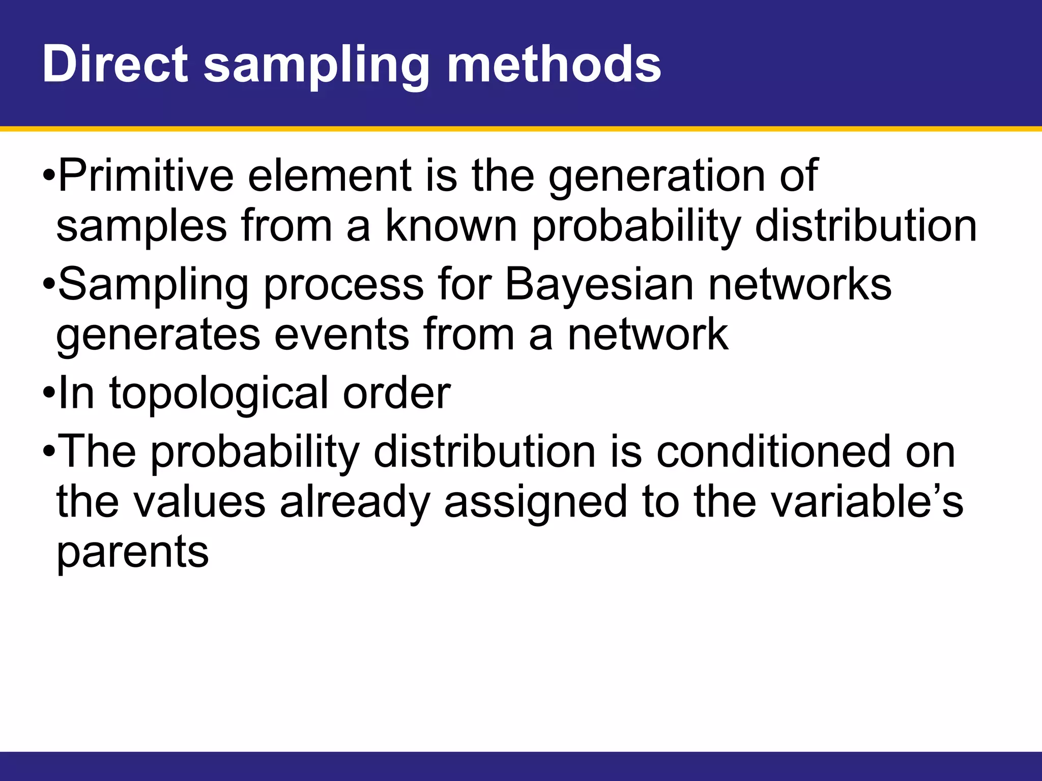
![Direct sampling methods
•Ex. Assuming an ordering
[Cloudy, Sprinkler, Rain, WetGrass]
1.Sample from P(Cloudy)
P(Cloudy) = <0.5, 0.5>
Cloudy = True](https://image.slidesharecdn.com/honyomich14-170519101244/75/Probabilistic-Reasoning-39-2048.jpg)
![Direct sampling methods
•Ex. Assuming an ordering
[Cloudy, Sprinkler, Rain, WetGrass]
2.Sample from P(Sprinkler|Cloudy=true)
P(S|C=true) = <0.1, 0.9>
Sprinkler = false](https://image.slidesharecdn.com/honyomich14-170519101244/75/Probabilistic-Reasoning-40-2048.jpg)
![Direct sampling methods
•Ex. Assuming an ordering
[Cloudy, Sprinkler, Rain, WetGrass]
3.Sample from P(Rain|Cloudy=true)
P(R|C=true) = <0.8, 0.2>
Rain = true](https://image.slidesharecdn.com/honyomich14-170519101244/75/Probabilistic-Reasoning-41-2048.jpg)
![Direct sampling methods
•Ex. Assuming an ordering
[Cloudy, Sprinkler, Rain, WetGrass]
4.Sample from P(W|S=false, R=true)
P(W|S=false, R=true) = <0.9, 0.1>
WetGrass = true
•In this case, the event
[Cloudy, Sprinkler, Rain, WetGrass]
= [true, false, true, true]](https://image.slidesharecdn.com/honyomich14-170519101244/75/Probabilistic-Reasoning-42-2048.jpg)
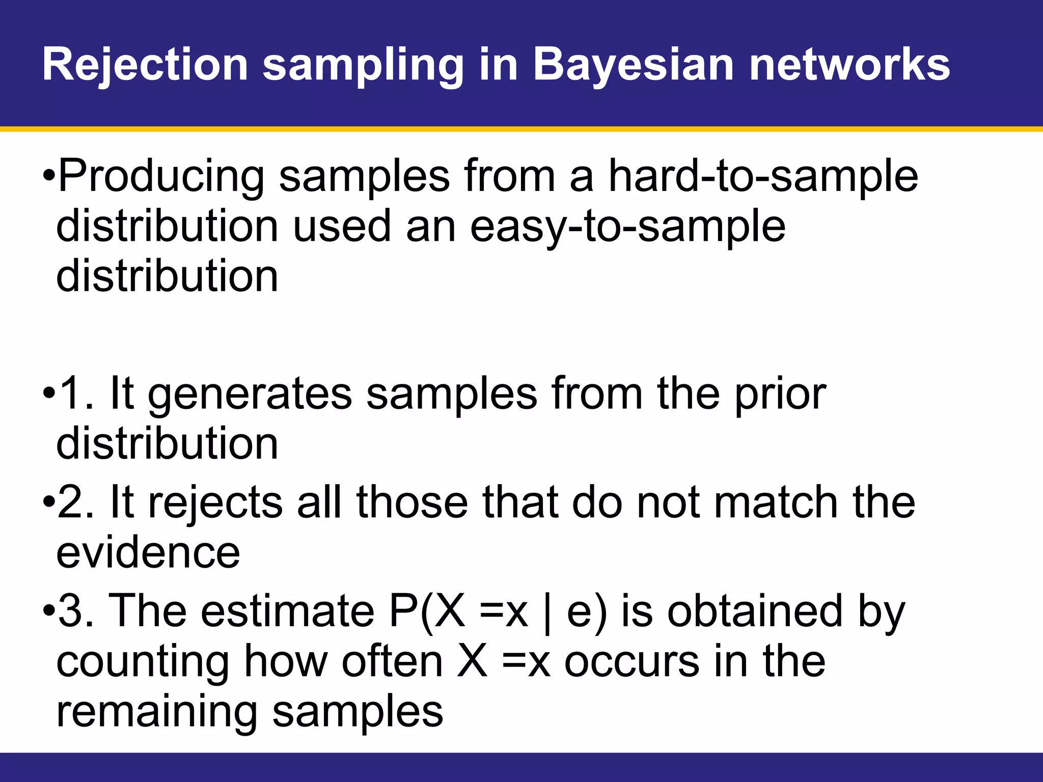


![Gibbs sampling in Bayesian networks
•Example
•P(Rain|Sprinkler = true, WetGrass = true)
oEvidence var = Sprinkler, WetGrass
oNonevidence var = Rain, Cloudy
o1.Arbitrarily initialize Rain and Cloudy(say true,
false)
[Cloudy, Sprinkler, Rain, WetGrass] = [T,T,F,T]](https://image.slidesharecdn.com/honyomich14-170519101244/75/Probabilistic-Reasoning-49-2048.jpg)
![Gibbs sampling in Bayesian networks
•Ex. Sampling
P(Rain|Sprinkler = true, WetGrass = true)
oCurrent state
[Cloudy, Sprinkler, Rain, WetGrass] = [T,T,F,T]
o2.Sample Cloudy
Its Markov’s blanket consists of Sprinkler, Rain.
Sample from P(Cloudy|Sprinkler=true, Rain=false)
Suppose we get false
Move to the next state with changed Cloudy
[Cloudy, Sprinkler, Rain, WetGrass] = [F,T,F,T]](https://image.slidesharecdn.com/honyomich14-170519101244/75/Probabilistic-Reasoning-50-2048.jpg)
![Gibbs sampling in Bayesian networks
•Ex. Sampling
P(Rain|Sprinkler = true, WetGrass = true)
oCurrent state
[Cloudy, Sprinkler, Rain, WetGrass] = [F,T,F,T]
o3.Sample Rain
Its Markov’s blanket consists of Sprinkler, Cloudy,
WetGrass.
Sample from
P(Rain|Sprinkler=true, Cloudy=false, WetGrass = true)
Suppose we get true.
Move to the next state with changed Cloudy
[Cloudy, Sprinkler, Rain, WetGrass] = [F,T,T,T]](https://image.slidesharecdn.com/honyomich14-170519101244/75/Probabilistic-Reasoning-51-2048.jpg)


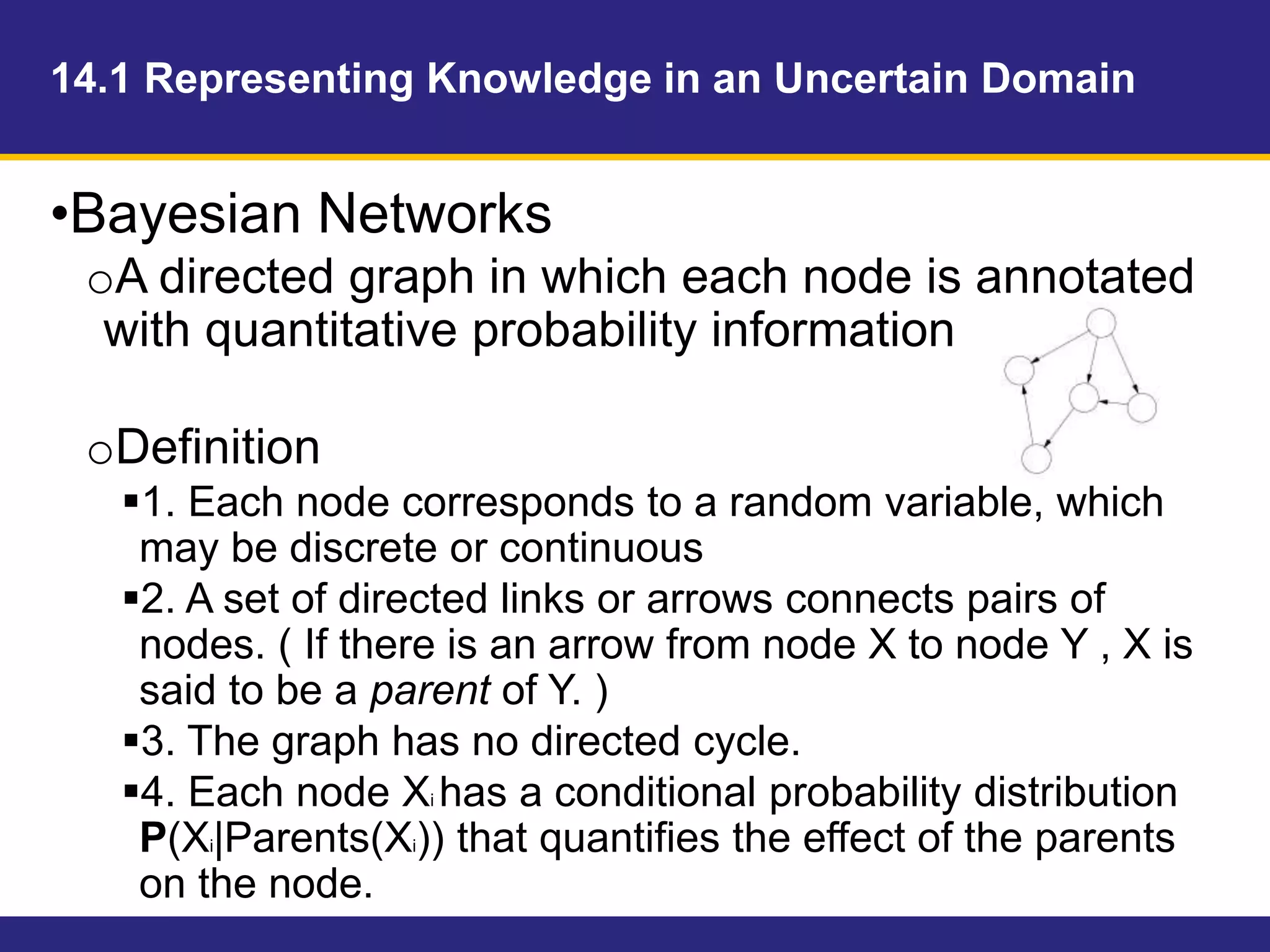
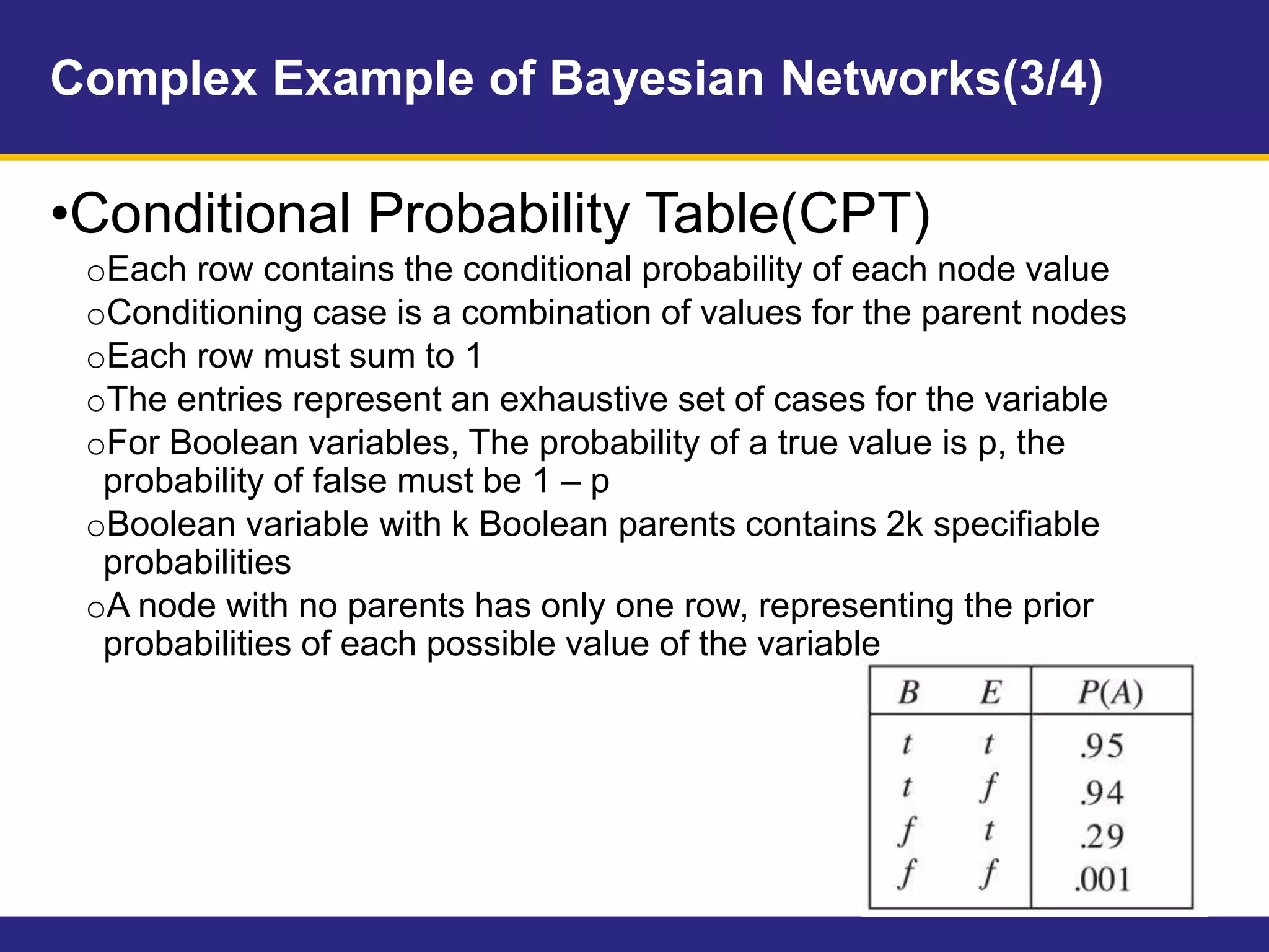
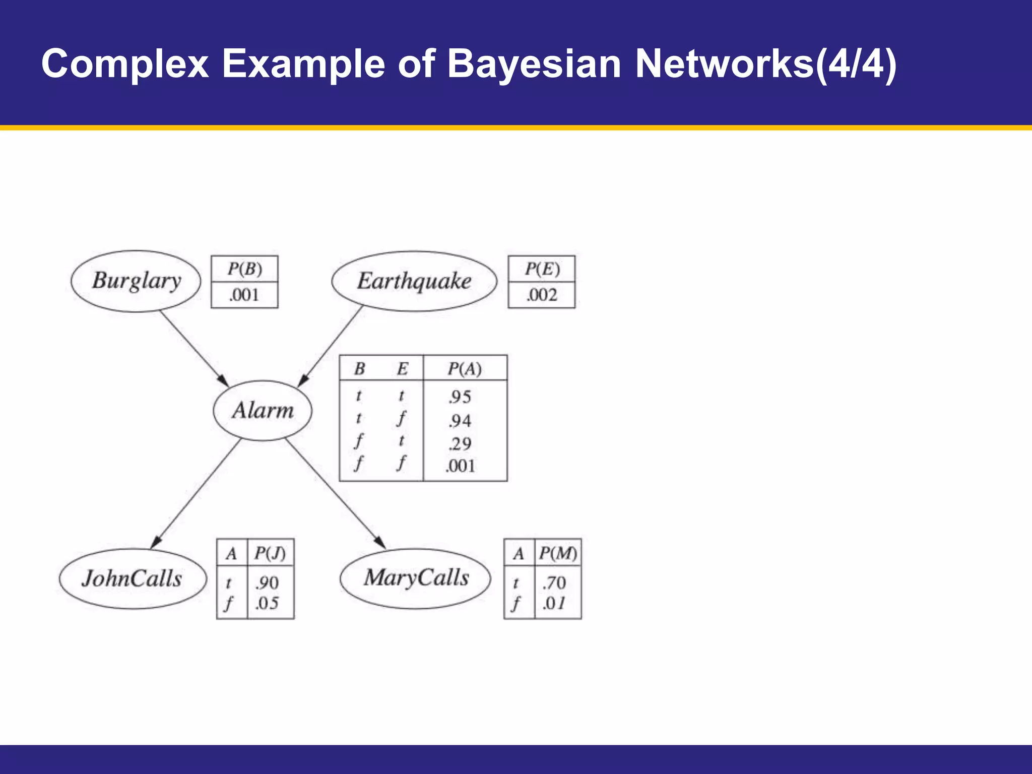
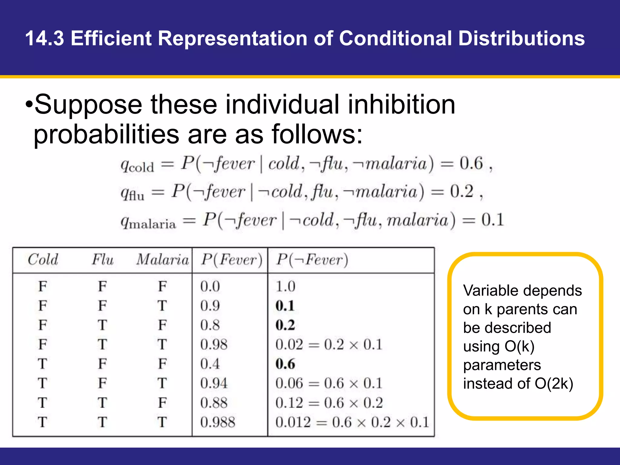
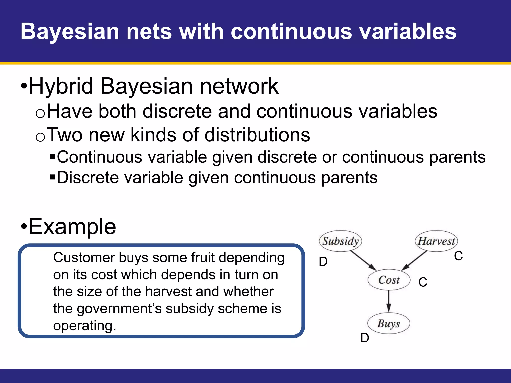
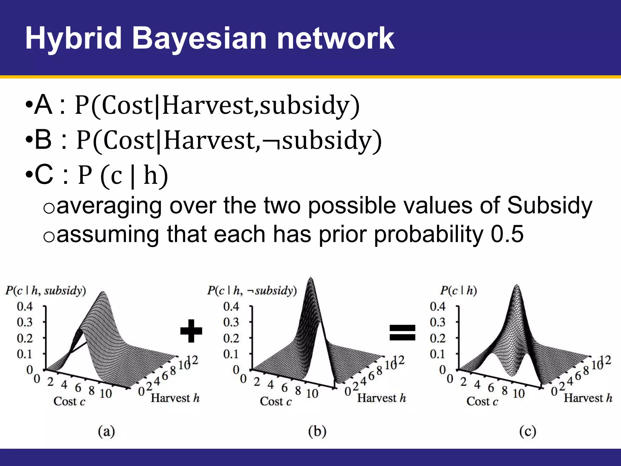
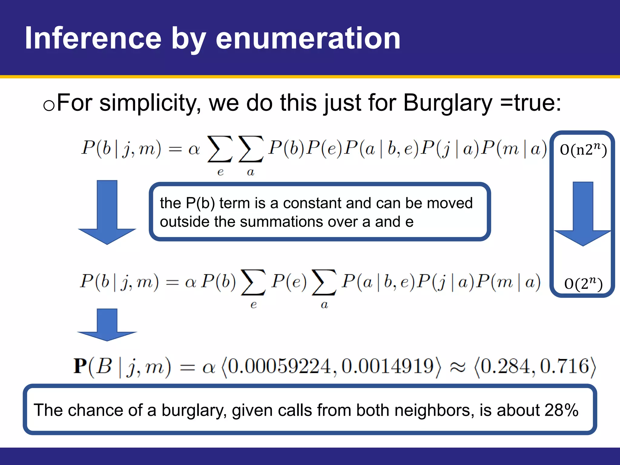
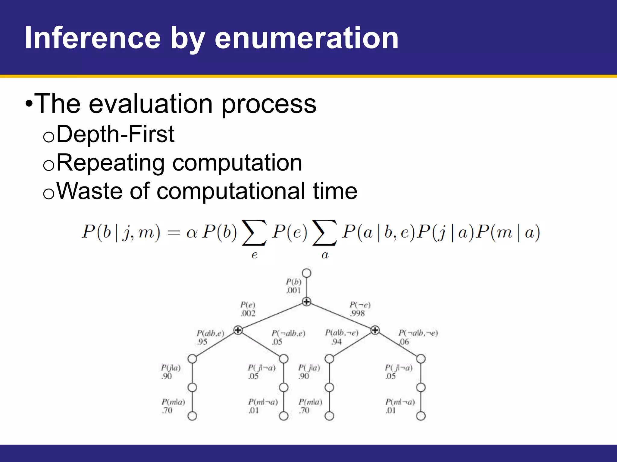
This document provides an overview of Chapter 14 on probabilistic reasoning and Bayesian networks from an artificial intelligence textbook. It introduces Bayesian networks as a way to represent knowledge over uncertain domains using directed graphs. Each node corresponds to a variable and arrows represent conditional dependencies between variables. The document explains how Bayesian networks can encode a joint probability distribution and represent conditional independence relationships. It also discusses techniques for efficiently representing conditional distributions in Bayesian networks, including noisy logical relationships and continuous variables. The chapter covers exact and approximate inference methods for Bayesian networks.