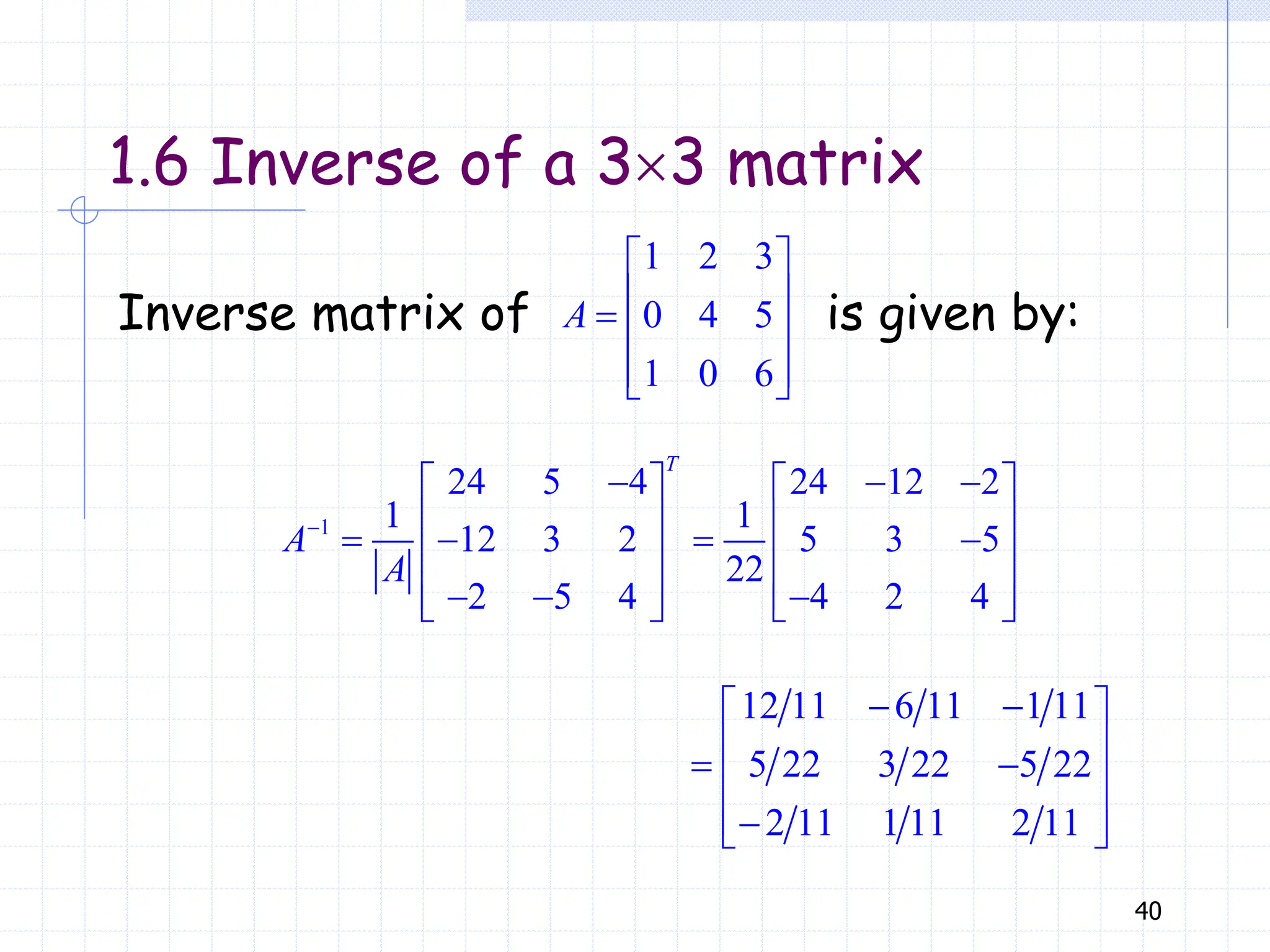
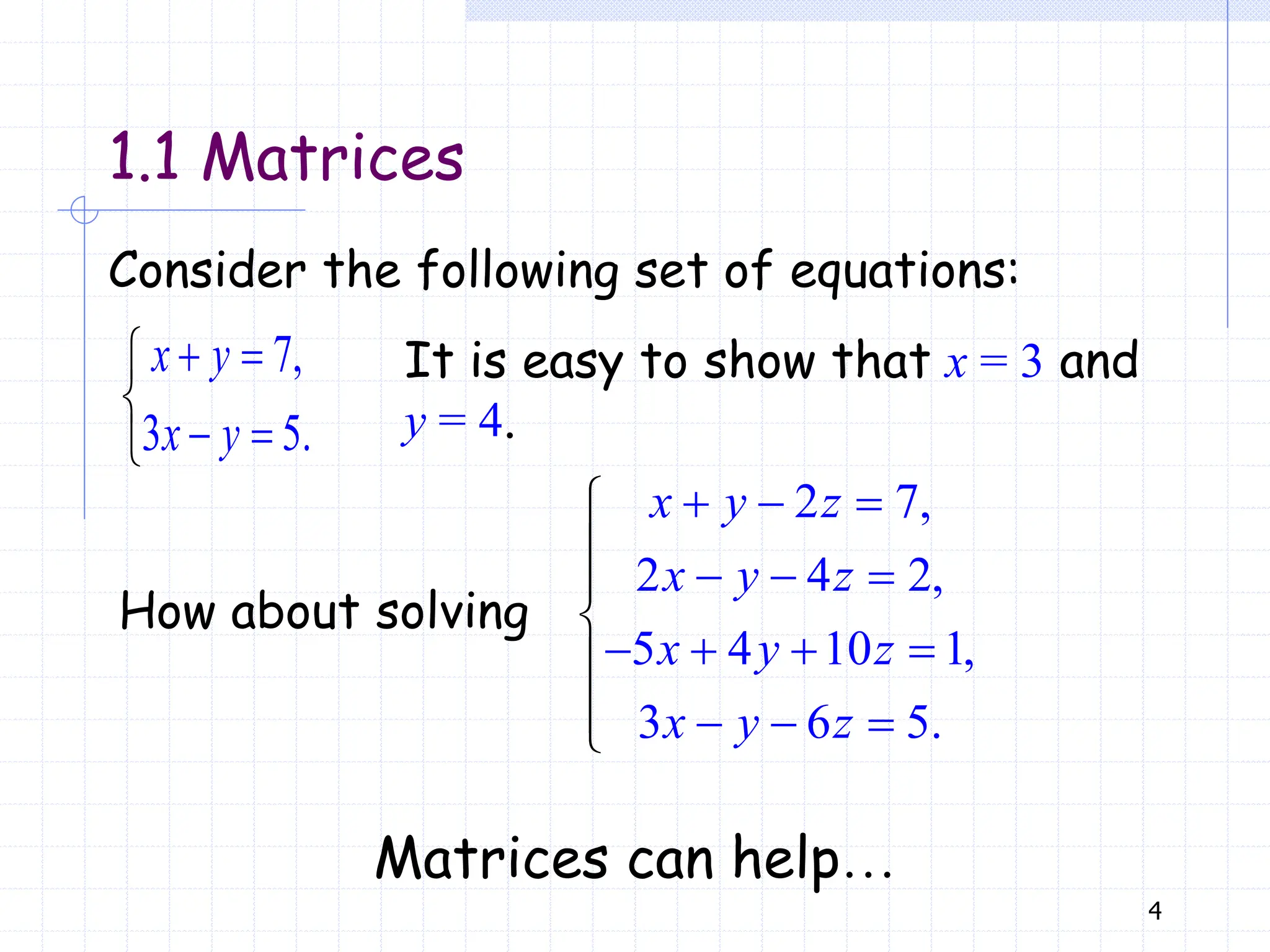
The document discusses matrices and determinants in detail, covering definitions, operations such as addition and multiplication, and properties of various types of matrices. It explains specific concepts such as square matrices, zero matrices, identity matrices, and explores scalar multiplication as well as the conditions for matrix equality. Additionally, it includes examples and properties related to the operations on matrices and their significance in mathematical computations.
![5
11 12 1
21 22 2
1 2
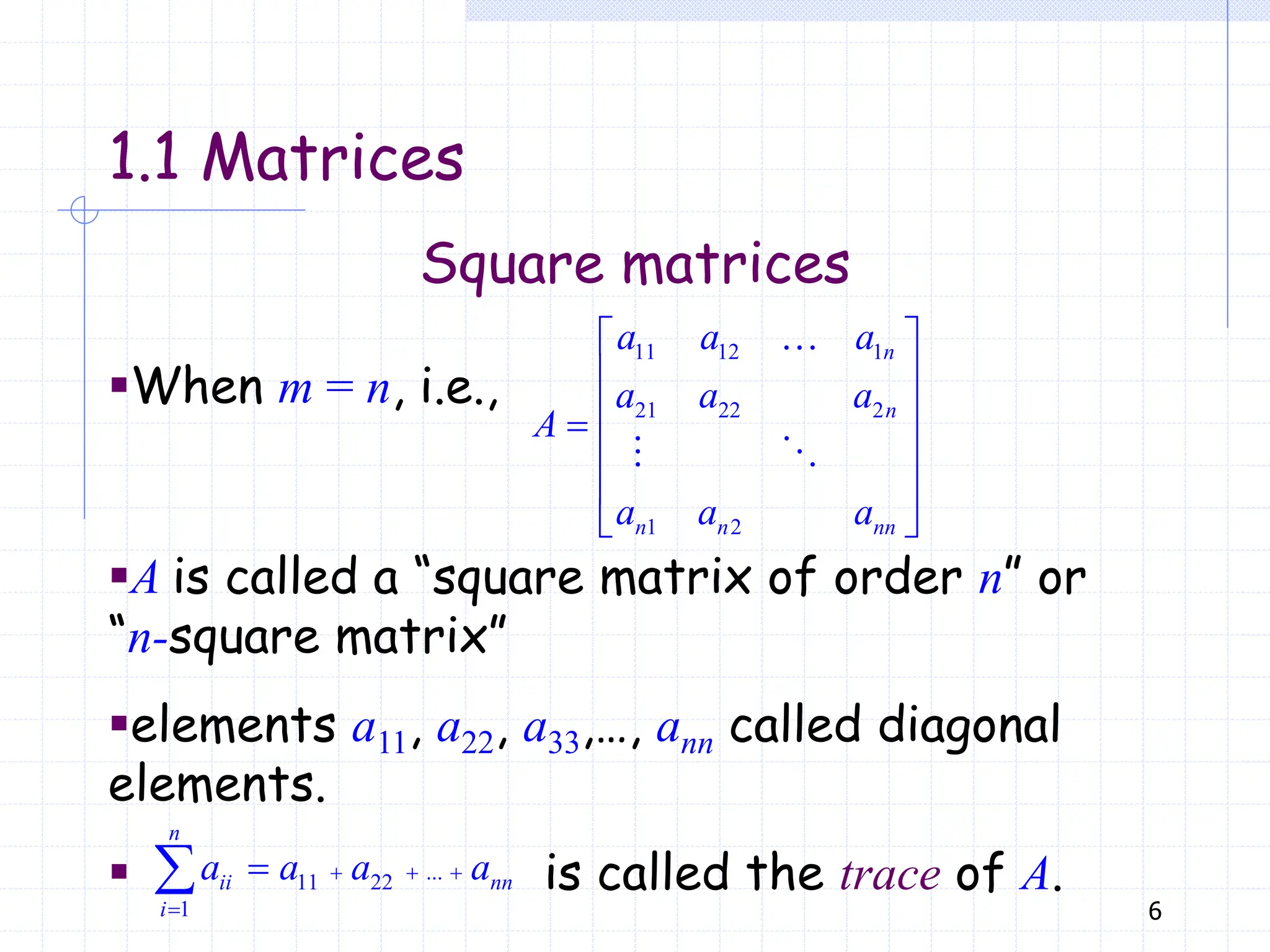
n
n
m m mn
a a a
a a a
A
a a a
In the matrix
▪numbers aij are called elements. First subscript
indicates the row; second subscript indicates
the column. The matrix consists of mn elements
▪It is called “the m n matrix A = [aij]” or simply
“the matrix A ” if number of rows and columns
are understood.
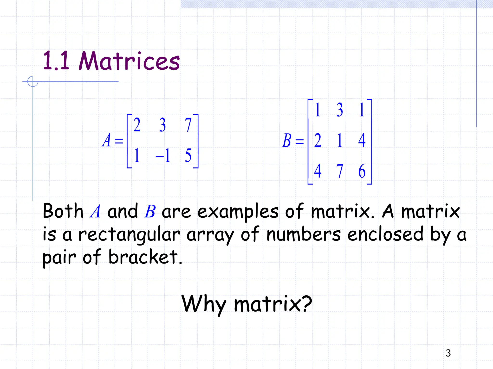
1.1 Matrices](https://image.slidesharecdn.com/ppt-physics-241015091415-4da5580b/75/ppt-power-point-presentation-physics-pdf-5-2048.jpg)
![7
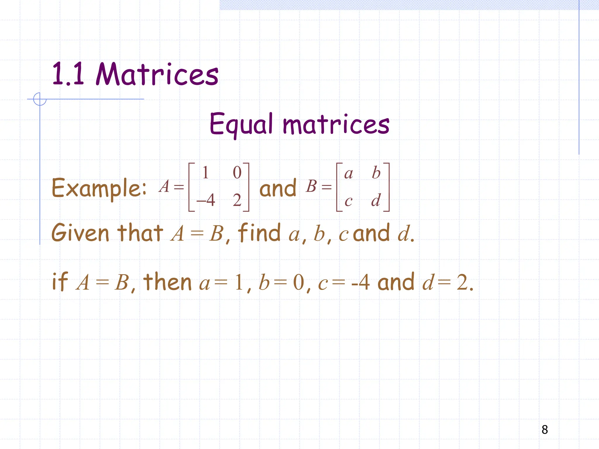
Equal matrices
▪Two matrices A = [aij] and B = [bij] are said to
be equal (A = B) iff each element of A is equal
to the corresponding element of B, i.e., aij = bij
for 1 i m, 1 j n.
▪iff pronouns “if and only if”
if A = B, it implies aij = bij for 1 i m, 1 j n;
if aij = bij for 1 i m, 1 j n, it implies A = B.
1.1 Matrices](https://image.slidesharecdn.com/ppt-physics-241015091415-4da5580b/75/ppt-power-point-presentation-physics-pdf-7-2048.jpg)
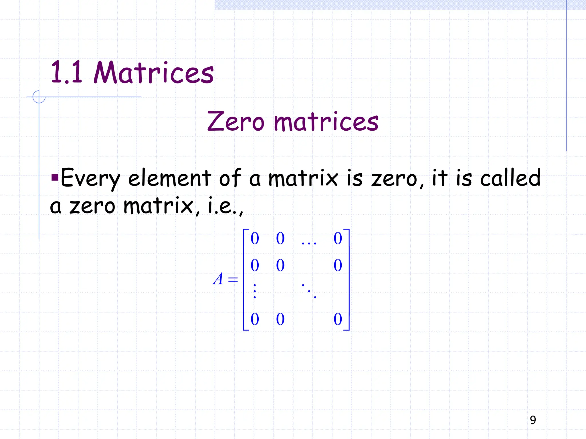
![10
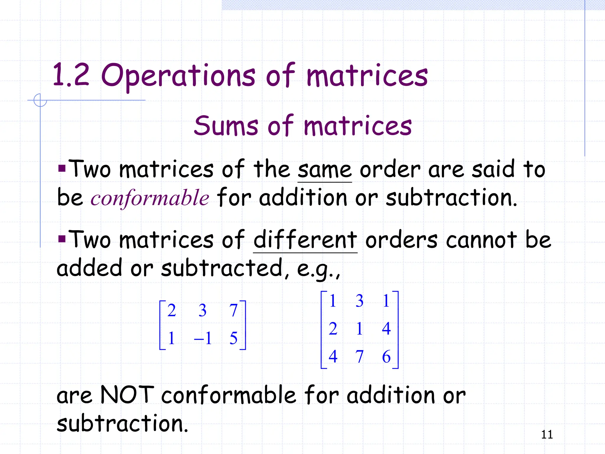
Sums of matrices
1.2 Operations of matrices
▪If A = [aij] and B = [bij] are m n matrices,
then A + B is defined as a matrix C = A + B,
where C= [cij], cij = aij + bij for 1 i m, 1 j n.
1 2 3
0 1 4
A
2 3 0
1 2 5
B
Example: if and
Evaluate A + B and A – B.
1 2 2 3 3 0 3 5 3
0 ( 1) 1 2 4 5 1 3 9
A B
1 2 2 3 3 0 1 1 3
0 ( 1) 1 2 4 5 1 1 1
A B](https://image.slidesharecdn.com/ppt-physics-241015091415-4da5580b/75/ppt-power-point-presentation-physics-pdf-10-2048.jpg)
![12
Scalar multiplication
1.2 Operations of matrices
▪Let l be any scalar and A = [aij] is an m n
matrix. Then lA = [laij] for 1 i m, 1 j n,
i.e., each element in A is multiplied by l.
1 2 3
0 1 4
A
Example: . Evaluate 3A.
3 1 3 2 3 3 3 6 9
3
3 0 3 1 3 4 0 3 12
A
▪In particular, l 1, i.e., A = [aij]. It’s called
the negative of A. Note: A A = 0 is a zero matrix](https://image.slidesharecdn.com/ppt-physics-241015091415-4da5580b/75/ppt-power-point-presentation-physics-pdf-12-2048.jpg)
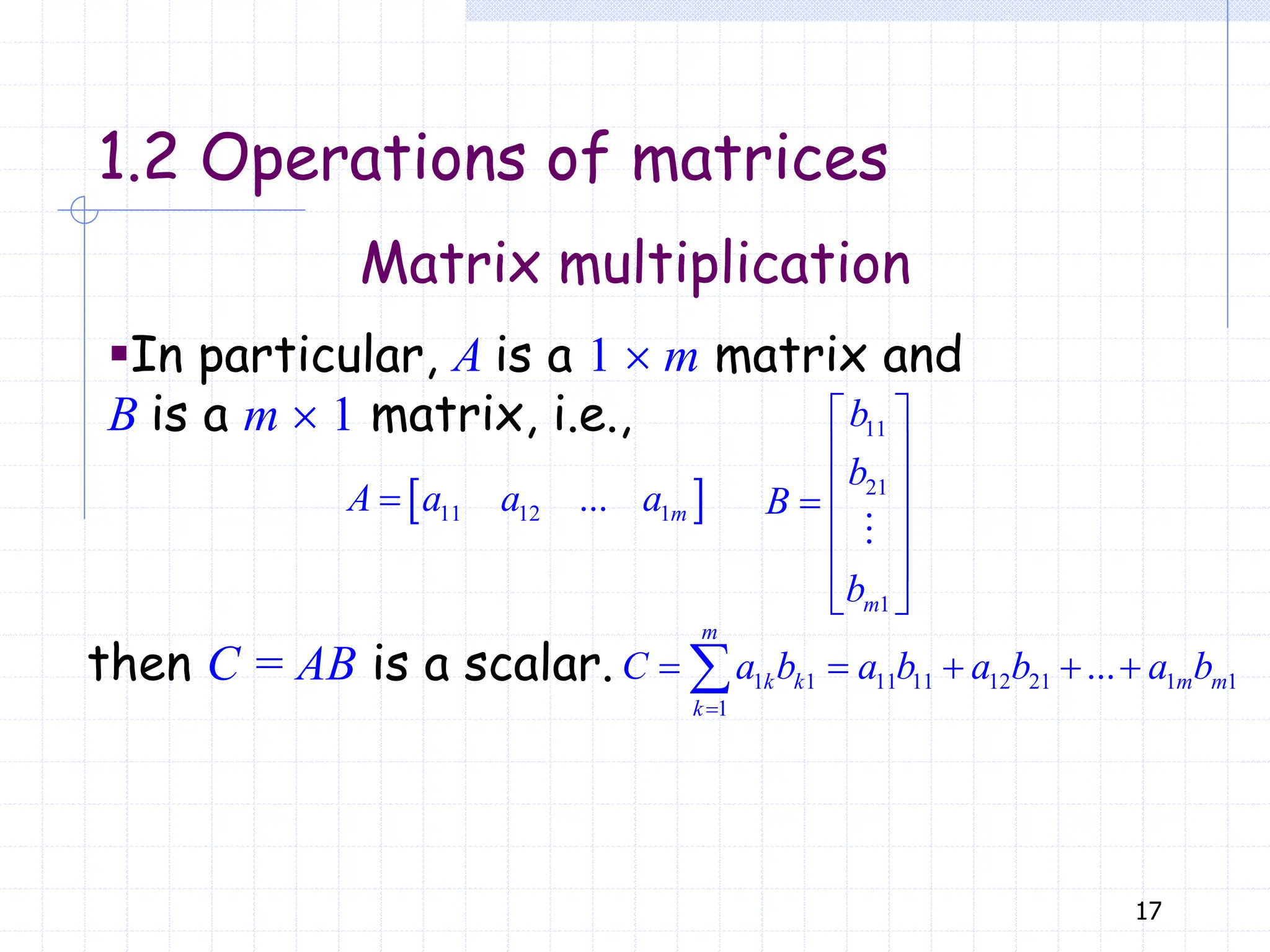
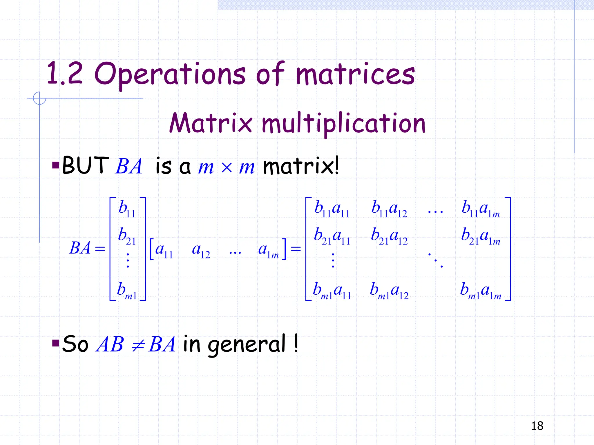
![15
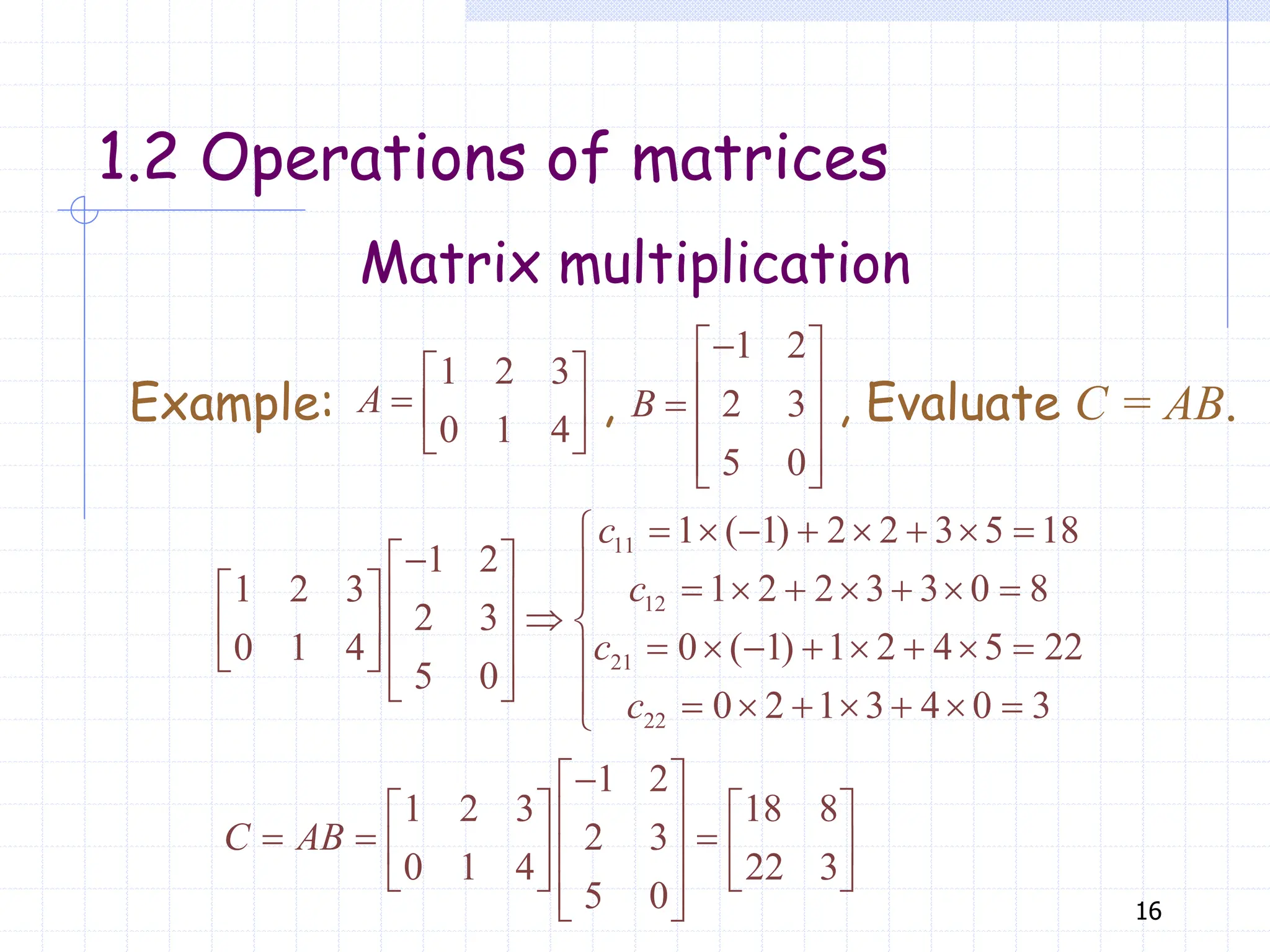
Matrix multiplication
1.2 Operations of matrices
▪If A = [aij] is a m p matrix and B = [bij] is a
p n matrix, then AB is defined as a m n
matrix C = AB, where C= [cij] with
1 1 2 2
1
...
p
ij ik kj i j i j ip pj
k
c a b a b a b a b
1 2 3
0 1 4
A
1 2
2 3
5 0
B
Example: , and C = AB.
Evaluate c21.
1 2
1 2 3
2 3
0 1 4
5 0
21 0 ( 1) 1 2 4 5 22
c
for 1 i m, 1 j n.](https://image.slidesharecdn.com/ppt-physics-241015091415-4da5580b/75/ppt-power-point-presentation-physics-pdf-15-2048.jpg)

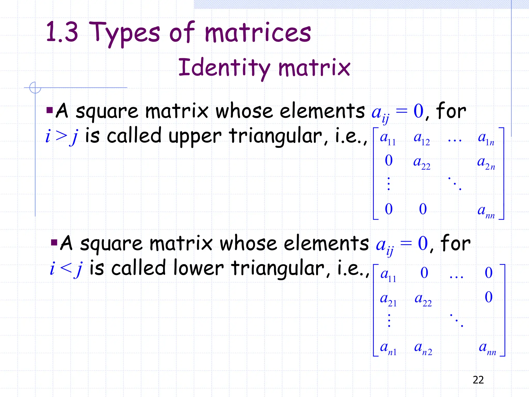
![23
▪Both upper and lower triangular, i.e., aij = 0, for
i j , i.e., 11
22
0 0
0 0
0 0
nn
a
a
D
a
11 22
diag[ , ,..., ]
nn
D a a a
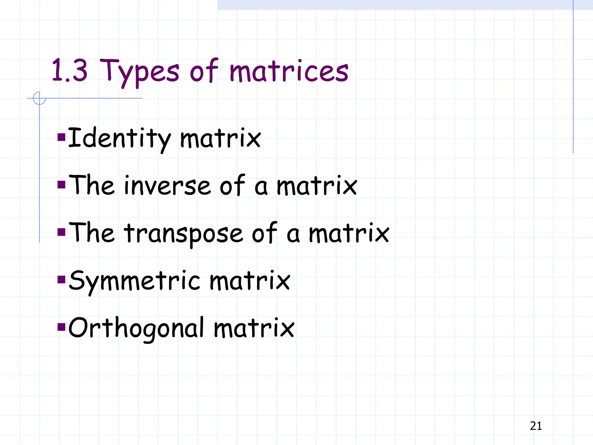
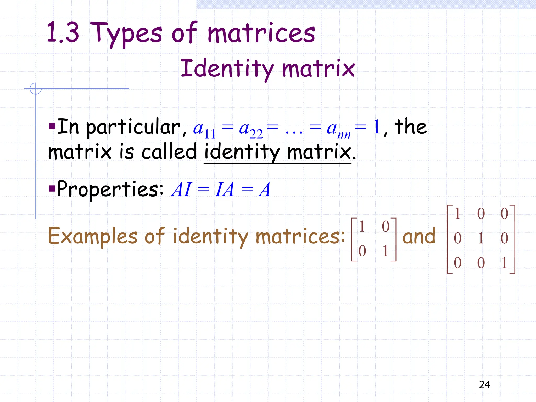
Identity matrix
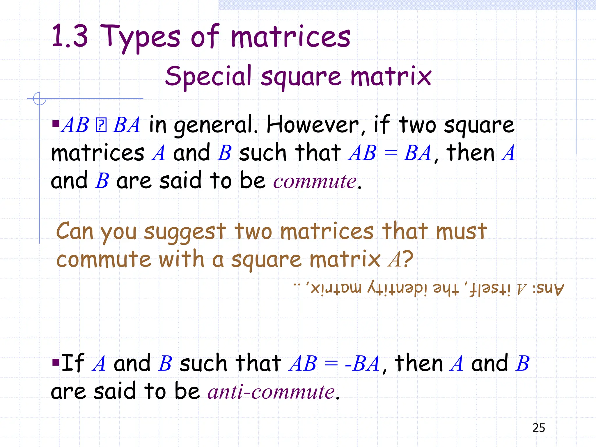
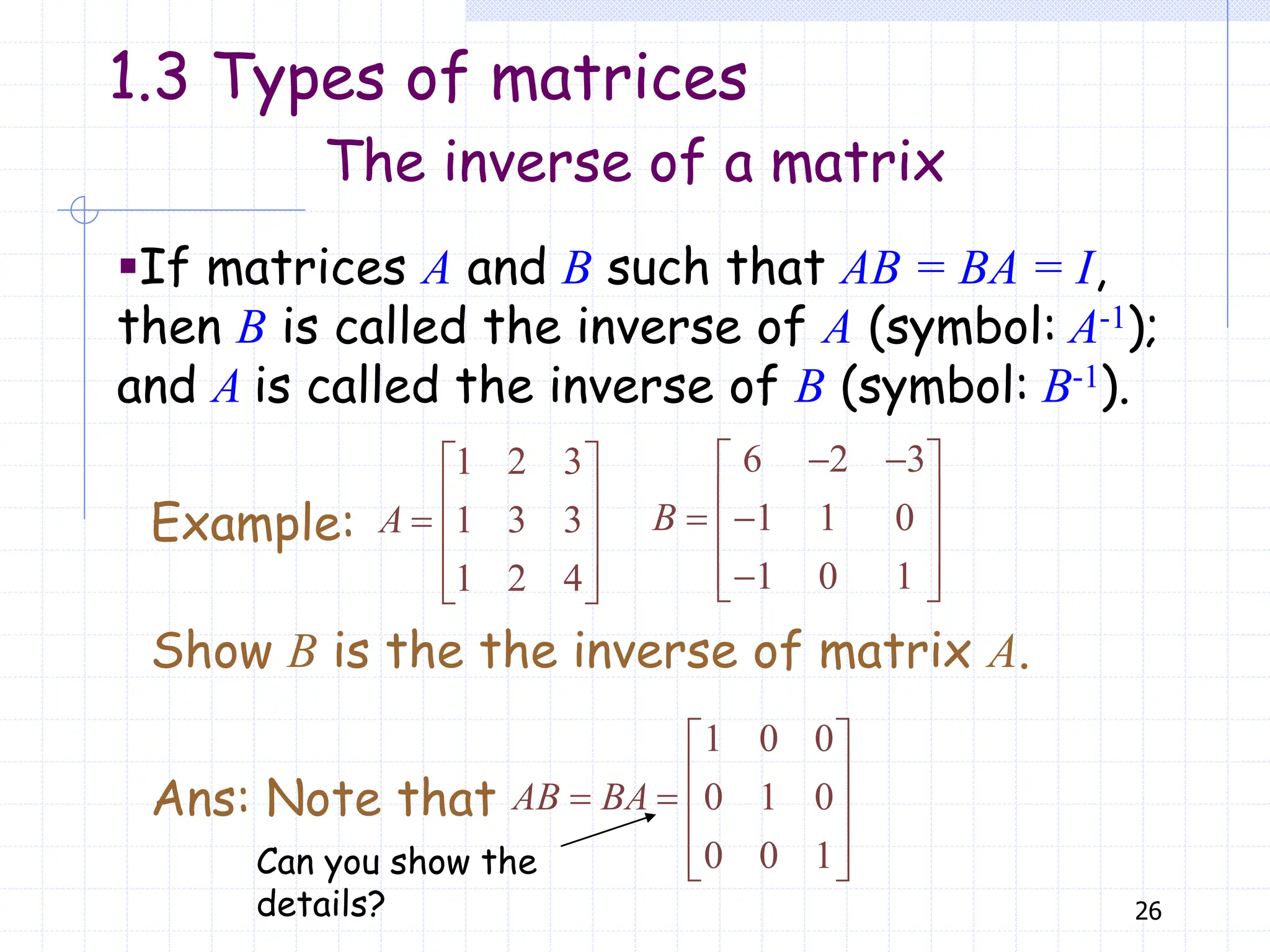
1.3 Types of matrices
is called a diagonal matrix, simply](https://image.slidesharecdn.com/ppt-physics-241015091415-4da5580b/75/ppt-power-point-presentation-physics-pdf-23-2048.jpg)
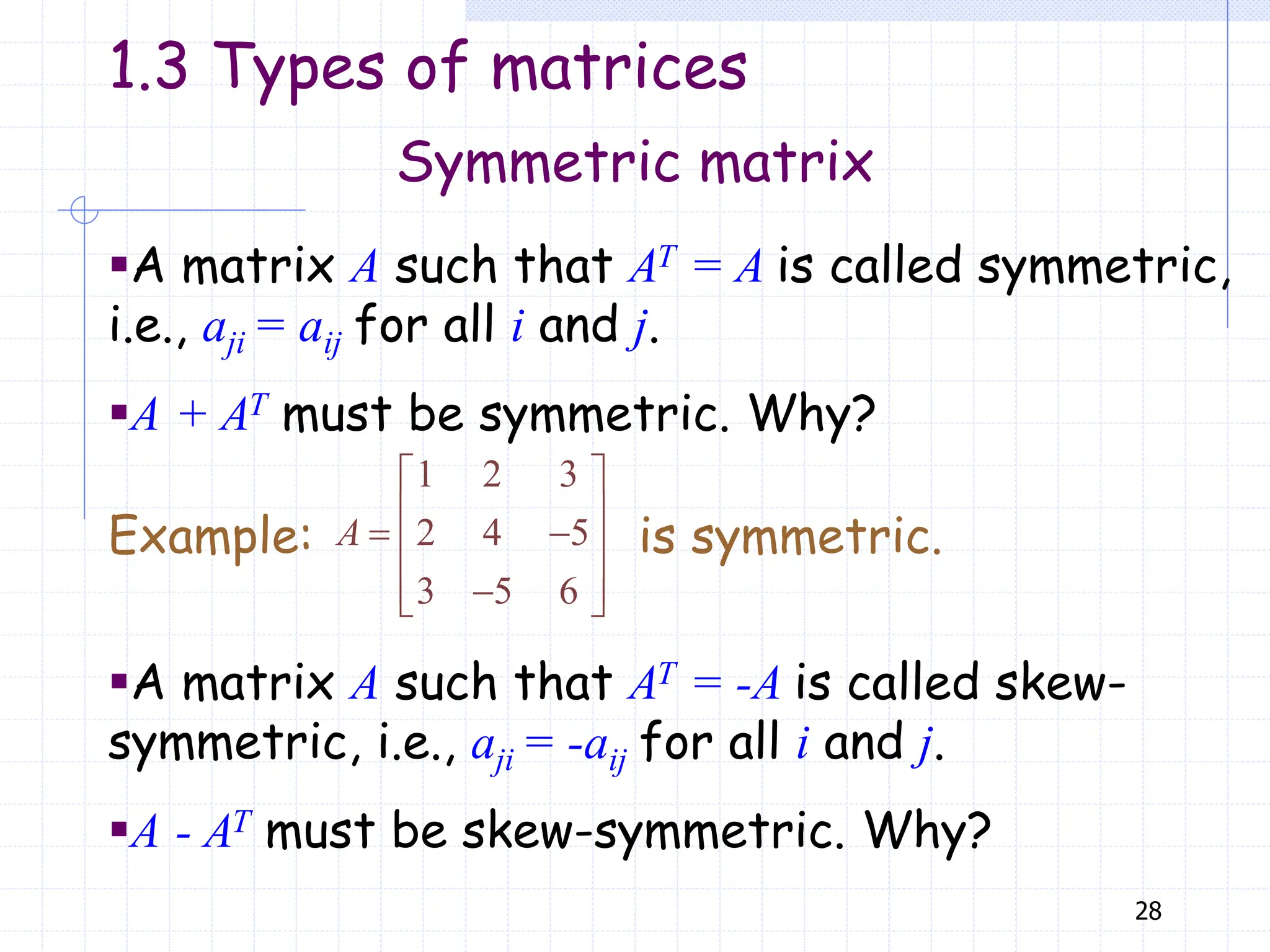
![27
The transpose of a matrix
▪The matrix obtained by interchanging the
rows and columns of a matrix A is called the
transpose of A (write AT).
Example:
The transpose of A is
1 2 3
4 5 6
A
1 4
2 5
3 6
T
A
▪For a matrix A = [aij], its transpose AT = [bij],
where bij = aji.
1.3 Types of matrices](https://image.slidesharecdn.com/ppt-physics-241015091415-4da5580b/75/ppt-power-point-presentation-physics-pdf-27-2048.jpg)