Introduction to Math for Artificial Introduction
Orthonormal Basis and Eigenvectors
Andres Mendez-Vazquez
March 23, 2020
1 / 127
Outline
1 Orthonormal Basis
Introduction
The Norm
The Row Space and Nullspace are Orthogonal sub-spaces inside Rn
Orthogonal Complements
Fundamental Theorems of Linear Algebra
Projections
Projection Onto a Subspace
Orthogonal Bases and Gram-Schmidt
Solving a Least Squared Error
The Gram Schmidt Process
The Gram Schmidt Algorithm and the QR Factorization
2 Eigenvectors
Introduction
What are eigenvector good for?
Modification on Distances
Relation with Invertibility
Finding Eigenvalues and Eigenvectors
Implications of Existence of Eigenvalues
Diagonalization of Matrices
Interesting Derivations
2 / 127
Outline
1 Orthonormal Basis
Introduction
The Norm
The Row Space and Nullspace are Orthogonal sub-spaces inside Rn
Orthogonal Complements
Fundamental Theorems of Linear Algebra
Projections
Projection Onto a Subspace
Orthogonal Bases and Gram-Schmidt
Solving a Least Squared Error
The Gram Schmidt Process
The Gram Schmidt Algorithm and the QR Factorization
2 Eigenvectors
Introduction
What are eigenvector good for?
Modification on Distances
Relation with Invertibility
Finding Eigenvalues and Eigenvectors
Implications of Existence of Eigenvalues
Diagonalization of Matrices
Interesting Derivations
3 / 127
The Dot Product
Definition
The dot product of two vectors v = [v1, v2, ..., vn]T
and
w = [w1, w2, ..., wn]T
v · w =
n
i=1
viwi
4 / 127
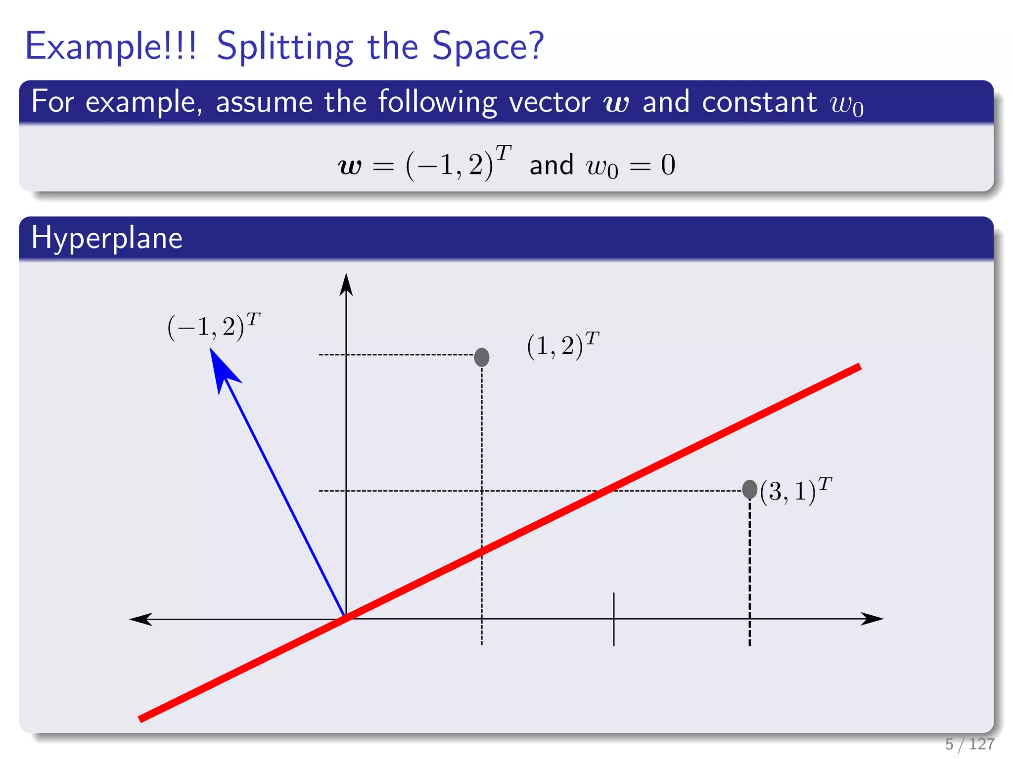
Example!!! Splitting the Space?
For example, assume the following vector w and constant w0
w = (−1, 2)T
and w0 = 0
Hyperplane
5 / 127
Example!!! Splitting the Space?
For example, assume the following vector w and constant w0
w = (−1, 2)T
and w0 = 0
Hyperplane
5 / 127
Then, we have
The following results
g
1
2
= (−1, 2)
1
2
= −1 × 1 + 2 × 2 = 3
g
3
1
= (−1, 2)
3
1
= −1 × 3 + 2 × 1 = −1
YES!!! We have a positive side and a negative side!!!
6 / 127
This product is also know as the Inner Product
Where
An inner product · · · , · · · satisfies the following four properties (u, v, w
vectors and α a escalar):
1 u + v, w = u, w + v, w
2 αv, w = α v, w
3 v, w = w, v
4 v, v ≥ 0 and equal to zero if v = 0.
7 / 127
Outline
1 Orthonormal Basis
Introduction
The Norm
The Row Space and Nullspace are Orthogonal sub-spaces inside Rn
Orthogonal Complements
Fundamental Theorems of Linear Algebra
Projections
Projection Onto a Subspace
Orthogonal Bases and Gram-Schmidt
Solving a Least Squared Error
The Gram Schmidt Process
The Gram Schmidt Algorithm and the QR Factorization
2 Eigenvectors
Introduction
What are eigenvector good for?
Modification on Distances
Relation with Invertibility
Finding Eigenvalues and Eigenvectors
Implications of Existence of Eigenvalues
Diagonalization of Matrices
Interesting Derivations
8 / 127
The Norm as a dot product
We can define the longitude of a vector
v =
√
v · v
A nice way to think about the longitude of a vector
9 / 127
The Norm as a dot product
We can define the longitude of a vector
v =
√
v · v
A nice way to think about the longitude of a vector
9 / 127
Orthogonal Vectors
We have that
Two vectors are orthogonal when their dot product is zero:
v · w = 0 or vT
w = 0
Remark
We want orthogonal bases and orthogonal sub-spaces.
10 / 127
Orthogonal Vectors
We have that
Two vectors are orthogonal when their dot product is zero:
v · w = 0 or vT
w = 0
Remark
We want orthogonal bases and orthogonal sub-spaces.
10 / 127
Some stuff about Row and Null Space
Something Notable
Every row of A is perpendicular to every solution of Ax = 0
In a similar way
Every column of A is perpendicular to every solution of AT x = 0
Meaning
What are the implications for the Column and Row Space?
11 / 127
Some stuff about Row and Null Space
Something Notable
Every row of A is perpendicular to every solution of Ax = 0
In a similar way
Every column of A is perpendicular to every solution of AT x = 0
Meaning
What are the implications for the Column and Row Space?
11 / 127
Some stuff about Row and Null Space
Something Notable
Every row of A is perpendicular to every solution of Ax = 0
In a similar way
Every column of A is perpendicular to every solution of AT x = 0
Meaning
What are the implications for the Column and Row Space?
11 / 127
Implications
We have that under Ax = b
e = b − Ax
Remember
The error at the Least Squared Error.
12 / 127
Implications
We have that under Ax = b
e = b − Ax
Remember
The error at the Least Squared Error.
12 / 127
Orthogonal Spaces
Definition
Two sub-spaces V and W of a vector space are orthogonal if every vector
v ∈ V is perpendicular to every vector w ∈ W.
In mathematical notation
vT
w = 0 ∀v ∈ V and ∀w ∈ W
13 / 127
Orthogonal Spaces
Definition
Two sub-spaces V and W of a vector space are orthogonal if every vector
v ∈ V is perpendicular to every vector w ∈ W.
In mathematical notation
vT
w = 0 ∀v ∈ V and ∀w ∈ W
13 / 127
Examples
At your Room
The floor of your room (extended to infinity) is a subspace V . The line
where two walls meet is a subspace W (one-dimensional).
A more convoluted example
Two walls look perpendicular but they are not orthogonal sub-spaces!
Why?
Any Idea?
14 / 127
Examples
At your Room
The floor of your room (extended to infinity) is a subspace V . The line
where two walls meet is a subspace W (one-dimensional).
A more convoluted example
Two walls look perpendicular but they are not orthogonal sub-spaces!
Why?
Any Idea?
14 / 127
Examples
At your Room
The floor of your room (extended to infinity) is a subspace V . The line
where two walls meet is a subspace W (one-dimensional).
A more convoluted example
Two walls look perpendicular but they are not orthogonal sub-spaces!
Why?
Any Idea?
14 / 127
For Example
Something Notable
15 / 127
Yes!!
The Line Shared by the Two Planes in R3
Therefore!!!
16 / 127
We have then
Theorem
The Null Space N (A) and the Row Space C AT , as the column space
of AT , are orthogonal sub-spaces in Rn
Proof
First, we have
Ax =






A1
A2
...
Am






x =






0
0
...
0






Therefore
Rows in A are perpendicular to x ⇒ Then x is also perpendicular to every
combination of the rows.
17 / 127
Then
Therefore
The whole row space is orthogonal to the N (A)
Better proof x ∈ N (A)- Hint What is AT
y?
x AT
y = (Ax)T
y = 0T
y = 0
AT y are all the possible combinations of the row space!!!
18 / 127
Then
Therefore
The whole row space is orthogonal to the N (A)
Better proof x ∈ N (A)- Hint What is AT
y?
x AT
y = (Ax)T
y = 0T
y = 0
AT y are all the possible combinations of the row space!!!
18 / 127
Then
Therefore
The whole row space is orthogonal to the N (A)
Better proof x ∈ N (A)- Hint What is AT
y?
x AT
y = (Ax)T
y = 0T
y = 0
AT y are all the possible combinations of the row space!!!
18 / 127
A little Bit of Notation
We use the following notation
N (A) ⊥ C AT
Definition
The orthogonal complement of a subspace V contains every vector that is
perpendicular to V .
This orthogonal subspace is denoted by
V ⊥
19 / 127
A little Bit of Notation
We use the following notation
N (A) ⊥ C AT
Definition
The orthogonal complement of a subspace V contains every vector that is
perpendicular to V .
This orthogonal subspace is denoted by
V ⊥
19 / 127
A little Bit of Notation
We use the following notation
N (A) ⊥ C AT
Definition
The orthogonal complement of a subspace V contains every vector that is
perpendicular to V .
This orthogonal subspace is denoted by
V ⊥
19 / 127
Thus, we have
Something Notable
By this definition, the nullspace is the orthogonal complement of the row
space.
20 / 127
Look at this
The Orthogonality
21 / 127
Orthogonal Complements
Definition
The orthogonal complement of a subspace V contains every vector
that is perpendicular to V .
This orthogonal subspace is denoted by V ⊥, pronounced “V prep”.
Something Notable
By this definition, the nullspace is the orthogonal complement of the row
space.
After All
Every x that is perpendicular to the rows satisfies Ax = 0.
22 / 127
Quite Interesting
We have the following
If v is orthogonal to the nullspace, it must be in the row space.
Therefore, we can build a new matrix
A =
A
v
Problem
The row space starts to grow and can break the law
dim (R(A)) + dim (Ker (A)) = n.
23 / 127
Quite Interesting
We have the following
If v is orthogonal to the nullspace, it must be in the row space.
Therefore, we can build a new matrix
A =
A
v
Problem
The row space starts to grow and can break the law
dim (R(A)) + dim (Ker (A)) = n.
23 / 127
Quite Interesting
We have the following
If v is orthogonal to the nullspace, it must be in the row space.
Therefore, we can build a new matrix
A =
A
v
Problem
The row space starts to grow and can break the law
dim (R(A)) + dim (Ker (A)) = n.
23 / 127
Additionally
The left nullspace and column space are orthogonal in Rm
Basically, they are orthogonal complements.
As always
Their dimensions dim Ker AT and dim R AT add to the full
dimension m.
24 / 127
Additionally
The left nullspace and column space are orthogonal in Rm
Basically, they are orthogonal complements.
As always
Their dimensions dim Ker AT and dim R AT add to the full
dimension m.
24 / 127
We have
Theorem
The column space and row space both have dimension r.
The nullspaces have dimensions n − r and m − r.
Theorem
The nullspace of A is the orthogonal complement of the row space
C AT - Rn.
Theorem
The null space of AT is the orthogonal complement of the column space
C (A) - Rm.
25 / 127
Splitting the Vectors
The point of "complements"
x can be split into a row space component xr and a nullspace component
xn:
x = xr + xn
Therefore
Ax = A [xr + xn] = Axr + Axn = Axr
Basically
Every vector goes to the column space.
26 / 127
Splitting the Vectors
The point of "complements"
x can be split into a row space component xr and a nullspace component
xn:
x = xr + xn
Therefore
Ax = A [xr + xn] = Axr + Axn = Axr
Basically
Every vector goes to the column space.
26 / 127
Splitting the Vectors
The point of "complements"
x can be split into a row space component xr and a nullspace component
xn:
x = xr + xn
Therefore
Ax = A [xr + xn] = Axr + Axn = Axr
Basically
Every vector goes to the column space.
26 / 127
Not only that
Every vector b in the column space
It comes from one and only one vector in the row space.
Proof
If Axr = Axr −→ the difference is in the nullspace xr − xr.
It is also in the row space...
Given that the nullspace and the row space are orthogonal.
They only share the vector 0.
27 / 127
Not only that
Every vector b in the column space
It comes from one and only one vector in the row space.
Proof
If Axr = Axr −→ the difference is in the nullspace xr − xr.
It is also in the row space...
Given that the nullspace and the row space are orthogonal.
They only share the vector 0.
27 / 127
Not only that
Every vector b in the column space
It comes from one and only one vector in the row space.
Proof
If Axr = Axr −→ the difference is in the nullspace xr − xr.
It is also in the row space...
Given that the nullspace and the row space are orthogonal.
They only share the vector 0.
27 / 127
Not only that
Every vector b in the column space
It comes from one and only one vector in the row space.
Proof
If Axr = Axr −→ the difference is in the nullspace xr − xr.
It is also in the row space...
Given that the nullspace and the row space are orthogonal.
They only share the vector 0.
27 / 127
Not only that
Every vector b in the column space
It comes from one and only one vector in the row space.
Proof
If Axr = Axr −→ the difference is in the nullspace xr − xr.
It is also in the row space...
Given that the nullspace and the row space are orthogonal.
They only share the vector 0.
27 / 127
And From Here
Something Notable
There is a r × r invertible matrix there hiding inside A.
If we throwaway the two nullspaces
From the row space to the column space, A is invertible
28 / 127
And From Here
Something Notable
There is a r × r invertible matrix there hiding inside A.
If we throwaway the two nullspaces
From the row space to the column space, A is invertible
28 / 127
Example
We have the matrix after echelon reduced
A =



3 0 0 0 0
0 5 0 0 0
0 0 0 0 0



You have the following invertible matrix
B =
3 0
0 5
29 / 127
Example
We have the matrix after echelon reduced
A =



3 0 0 0 0
0 5 0 0 0
0 0 0 0 0



You have the following invertible matrix
B =
3 0
0 5
29 / 127
Outline
1 Orthonormal Basis
Introduction
The Norm
The Row Space and Nullspace are Orthogonal sub-spaces inside Rn
Orthogonal Complements
Fundamental Theorems of Linear Algebra
Projections
Projection Onto a Subspace
Orthogonal Bases and Gram-Schmidt
Solving a Least Squared Error
The Gram Schmidt Process
The Gram Schmidt Algorithm and the QR Factorization
2 Eigenvectors
Introduction
What are eigenvector good for?
Modification on Distances
Relation with Invertibility
Finding Eigenvalues and Eigenvectors
Implications of Existence of Eigenvalues
Diagonalization of Matrices
Interesting Derivations
30 / 127
Assume that you are in R3
Something like
31 / 127
Simple but complex
A simple question
What are the projections of b = (2, 3, 4) onto the z axis and the xy
plane?
Can we use matrices to talk about these projections?
First
We must have a projection matrix P with the following property:
P2
= P
Why?
Ideas?
32 / 127
Simple but complex
A simple question
What are the projections of b = (2, 3, 4) onto the z axis and the xy
plane?
Can we use matrices to talk about these projections?
First
We must have a projection matrix P with the following property:
P2
= P
Why?
Ideas?
32 / 127
Simple but complex
A simple question
What are the projections of b = (2, 3, 4) onto the z axis and the xy
plane?
Can we use matrices to talk about these projections?
First
We must have a projection matrix P with the following property:
P2
= P
Why?
Ideas?
32 / 127
Then, the Projection Pb
First
When b is projected onto a line, its projection p is the part of b along that
line.
Second
When b is projected onto a plane, its projection p is the part of the plane.
33 / 127
Then, the Projection Pb
First
When b is projected onto a line, its projection p is the part of b along that
line.
Second
When b is projected onto a plane, its projection p is the part of the plane.
33 / 127
In our case
The Projection Matrices for the coordinate systems
P1 =



0 0 0
0 0 0
0 0 1


 , P2 =



0 0 0
0 1 0
0 0 0


 , P3 =



1 0 0
0 0 0
0 0 0



34 / 127
Example
We have the following vector b = (2, 3, 4)T
Onto the z axis:
P1b =



0 0 0
0 0 0
0 0 1






2
3
4


 =



0
0
4



What about the plane xy
Any idea?
35 / 127
Example
We have the following vector b = (2, 3, 4)T
Onto the z axis:
P1b =



0 0 0
0 0 0
0 0 1






2
3
4


 =



0
0
4



What about the plane xy
Any idea?
35 / 127
We have something more complex
Something Notable
P4 =



1 0 0
0 1 0
0 0 0



Then
P4b =



1 0 0
0 1 0
0 0 0






2
3
4


 =



2
3
0



36 / 127
We have something more complex
Something Notable
P4 =



1 0 0
0 1 0
0 0 0



Then
P4b =



1 0 0
0 1 0
0 0 0






2
3
4


 =



2
3
0



36 / 127
Assume the following
We have that
a1, a2, ..., an in Rm.
Assume they are linearly independent
They span a subspace, we want projections into the subspace
We want to project b into such subspace
How do we do it?
37 / 127
Assume the following
We have that
a1, a2, ..., an in Rm.
Assume they are linearly independent
They span a subspace, we want projections into the subspace
We want to project b into such subspace
How do we do it?
37 / 127
Assume the following
We have that
a1, a2, ..., an in Rm.
Assume they are linearly independent
They span a subspace, we want projections into the subspace
We want to project b into such subspace
How do we do it?
37 / 127
This is the important part
Problem
Find the combination p = x1a1 + x2a2 + · · · + xnan closest to vector b.
Something Notable
With n = 1 (only one vector a1) this projection onto a line.
This line is the column space of A
Basically the columns are spanned by a single column.
38 / 127
This is the important part
Problem
Find the combination p = x1a1 + x2a2 + · · · + xnan closest to vector b.
Something Notable
With n = 1 (only one vector a1) this projection onto a line.
This line is the column space of A
Basically the columns are spanned by a single column.
38 / 127
This is the important part
Problem
Find the combination p = x1a1 + x2a2 + · · · + xnan closest to vector b.
Something Notable
With n = 1 (only one vector a1) this projection onto a line.
This line is the column space of A
Basically the columns are spanned by a single column.
38 / 127
In General
The matrix has n columns a1, a2, ..., an
The combinations in Rm are vectors Ax in the column space
We are looking for the particular combination
The nearest to the original b
p = Ax
39 / 127
In General
The matrix has n columns a1, a2, ..., an
The combinations in Rm are vectors Ax in the column space
We are looking for the particular combination
The nearest to the original b
p = Ax
39 / 127
First
We look at the simplest case
The projection into a line...
40 / 127
With a little of Geometry
We have the following
Projection
0
41 / 127
Therefore
Using the fact that the projection is equal to
p = xa
Then, the error is equal to
e = b − xa
We have that a · e = 0
a · e = a · (b − xa) = a · b − xa · a = 0
42 / 127
Therefore
Using the fact that the projection is equal to
p = xa
Then, the error is equal to
e = b − xa
We have that a · e = 0
a · e = a · (b − xa) = a · b − xa · a = 0
42 / 127
Therefore
Using the fact that the projection is equal to
p = xa
Then, the error is equal to
e = b − xa
We have that a · e = 0
a · e = a · (b − xa) = a · b − xa · a = 0
42 / 127
Therefore
We have that
x =
a · b
a · a
=
aT b
aT a
Or something quite simple
p =
aT b
aT a
a
43 / 127
Therefore
We have that
x =
a · b
a · a
=
aT b
aT a
Or something quite simple
p =
aT b
aT a
a
43 / 127
By the Law of Cosines
Something Notable
a − b 2
= a 2
+ b 2
− 2 a b cos Θ
44 / 127
We have
The following product
a · a − 2a · b + b · b = a 2
+ b 2
− 2 a b cos Θ
Then
a · b = a b cos Θ
45 / 127
We have
The following product
a · a − 2a · b + b · b = a 2
+ b 2
− 2 a b cos Θ
Then
a · b = a b cos Θ
45 / 127
With Length
Using the Norm
p =
aT b
aT a
a =
a b cos Θ
a 2 a = b |cos Θ|
46 / 127
Example
Project
b =



1
1
1


 onto a =



1
2
2



Find
p = xa
47 / 127
Example
Project
b =



1
1
1


 onto a =



1
2
2



Find
p = xa
47 / 127
What about the Projection Matrix in general
We have
p = ax =
aaT b
aT a
= Pb
Then
P =
aaT
aT a
48 / 127
What about the Projection Matrix in general
We have
p = ax =
aaT b
aT a
= Pb
Then
P =
aaT
aT a
48 / 127
Example
Find the projection matrix for
b =



1
1
1


 onto a =



1
2
2



49 / 127
What about the general case?
We have that
Find the combination p = x1a1 + x2a2 + · · · + xnan closest to vector b.
Now you need a vector
Find the vector x,find the projection p = Ax,find the matrix P.
Again, the error is perpendicular to the space
e = b − Ax
50 / 127
What about the general case?
We have that
Find the combination p = x1a1 + x2a2 + · · · + xnan closest to vector b.
Now you need a vector
Find the vector x,find the projection p = Ax,find the matrix P.
Again, the error is perpendicular to the space
e = b − Ax
50 / 127
What about the general case?
We have that
Find the combination p = x1a1 + x2a2 + · · · + xnan closest to vector b.
Now you need a vector
Find the vector x,find the projection p = Ax,find the matrix P.
Again, the error is perpendicular to the space
e = b − Ax
50 / 127
Therefore
The error e = b − Ax
aT
1 (b − Ax) = 0
...
...
aT
n (b − Ax) = 0
Or



aT
1
...
aT
n


 [b − Ax] = 0
51 / 127
Therefore
The error e = b − Ax
aT
1 (b − Ax) = 0
...
...
aT
n (b − Ax) = 0
Or



aT
1
...
aT
n


 [b − Ax] = 0
51 / 127
Therefore
The Matrix with those rows is AT
AT
(b − Ax) = 0
Therefore
AT
b − AT
Ax = 0
Or the most know form
x = AT
A
−1
AT
b
52 / 127
Therefore
The Matrix with those rows is AT
AT
(b − Ax) = 0
Therefore
AT
b − AT
Ax = 0
Or the most know form
x = AT
A
−1
AT
b
52 / 127
Therefore
The Matrix with those rows is AT
AT
(b − Ax) = 0
Therefore
AT
b − AT
Ax = 0
Or the most know form
x = AT
A
−1
AT
b
52 / 127
Therefore
The Projection is
p = Ax = A AT
A
−1
AT
b
Therefore
P = A AT
A
−1
AT
53 / 127
Therefore
The Projection is
p = Ax = A AT
A
−1
AT
b
Therefore
P = A AT
A
−1
AT
53 / 127
The key step was AT
[b − Ax] = 0
Linear algebra gives this "normal equation"
1 Our subspace is the column space of A.
2 The error vector b − Ax is perpendicular to that column space.
3 Therefore b − Ax is in the nullspace of AT
54 / 127
When A has independent columns, AT
A is invertible
Theorem
AT A is invertible if and only if Ahas linearly independent columns.
55 / 127
Proof
Consider the following
AT
Ax = 0
Here, Ax is in the null space of AT
Remember the column space and null space of AT are orthogonal
complements.
And Ax an element in the column space of A
Ax = 0
56 / 127
Proof
Consider the following
AT
Ax = 0
Here, Ax is in the null space of AT
Remember the column space and null space of AT are orthogonal
complements.
And Ax an element in the column space of A
Ax = 0
56 / 127
Proof
Consider the following
AT
Ax = 0
Here, Ax is in the null space of AT
Remember the column space and null space of AT are orthogonal
complements.
And Ax an element in the column space of A
Ax = 0
56 / 127
Proof
If A has linearly independent columns
Ax = 0 =⇒ x = 0
Then, the null space
Null AT
A = {0}
i.e AT
A is full rank
Then, AT A is invertible...
57 / 127
Proof
If A has linearly independent columns
Ax = 0 =⇒ x = 0
Then, the null space
Null AT
A = {0}
i.e AT
A is full rank
Then, AT A is invertible...
57 / 127
Proof
If A has linearly independent columns
Ax = 0 =⇒ x = 0
Then, the null space
Null AT
A = {0}
i.e AT
A is full rank
Then, AT A is invertible...
57 / 127
Finally
Theorem
When A has independent columns, AT
A is square, symmetric
and invertible.
58 / 127
Example
Use Gauss-Jordan for finding if AT
A is invertible
A =



1 2
1 2
0 0



59 / 127
Example
Given
A =



1 0
1 1
1 2


 and b =



6
0
0



Find
x and p and P
60 / 127
Example
Given
A =



1 0
1 1
1 2


 and b =



6
0
0



Find
x and p and P
60 / 127
Outline
1 Orthonormal Basis
Introduction
The Norm
The Row Space and Nullspace are Orthogonal sub-spaces inside Rn
Orthogonal Complements
Fundamental Theorems of Linear Algebra
Projections
Projection Onto a Subspace
Orthogonal Bases and Gram-Schmidt
Solving a Least Squared Error
The Gram Schmidt Process
The Gram Schmidt Algorithm and the QR Factorization
2 Eigenvectors
Introduction
What are eigenvector good for?
Modification on Distances
Relation with Invertibility
Finding Eigenvalues and Eigenvectors
Implications of Existence of Eigenvalues
Diagonalization of Matrices
Interesting Derivations
61 / 127
Now, we always like to make our life easier
Something Notable
Orthogonality makes easier to find x, p and P.
For this, we will find the orthogonal vectors
At the column space of A
62 / 127
Now, we always like to make our life easier
Something Notable
Orthogonality makes easier to find x, p and P.
For this, we will find the orthogonal vectors
At the column space of A
62 / 127
Orthonormal Vectors
Definition
The vectors q1, q2, ..., qn are orthonormal if
qT
i qj =
0 when i = j
1 when i = j
Then
A matrix with orthonormal columns is assigned the special letter Q
Properties
A matrix Q with orthonormal columns satisfies QT Q = I
63 / 127
Orthonormal Vectors
Definition
The vectors q1, q2, ..., qn are orthonormal if
qT
i qj =
0 when i = j
1 when i = j
Then
A matrix with orthonormal columns is assigned the special letter Q
Properties
A matrix Q with orthonormal columns satisfies QT Q = I
63 / 127
Orthonormal Vectors
Definition
The vectors q1, q2, ..., qn are orthonormal if
qT
i qj =
0 when i = j
1 when i = j
Then
A matrix with orthonormal columns is assigned the special letter Q
Properties
A matrix Q with orthonormal columns satisfies QT Q = I
63 / 127
Additionally
Given that
QT
Q = I
Therefore
When Q is square, QT Q = I means that QT = Q−1: transpose = inverse.
64 / 127
Additionally
Given that
QT
Q = I
Therefore
When Q is square, QT Q = I means that QT = Q−1: transpose = inverse.
64 / 127
Examples
Rotation
cos Θ − sin Θ
sin Θ cos Θ
Permutation Matrix
0 1
1 0
Reflection
Setting Q = I − 2uuT with u a unit vector.
65 / 127
Examples
Rotation
cos Θ − sin Θ
sin Θ cos Θ
Permutation Matrix
0 1
1 0
Reflection
Setting Q = I − 2uuT with u a unit vector.
65 / 127
Examples
Rotation
cos Θ − sin Θ
sin Θ cos Θ
Permutation Matrix
0 1
1 0
Reflection
Setting Q = I − 2uuT with u a unit vector.
65 / 127
Finally
If Q has orthonormal columns
The lengths are unchanged
How?
Qx = xT QT Qx =
√
xT x = x
66 / 127
Finally
If Q has orthonormal columns
The lengths are unchanged
How?
Qx = xT QT Qx =
√
xT x = x
66 / 127
Remark
Something Notable
When the columns of A were a basis for the subspace.
All Formulas involve
AT
A
What happens when the basis vectors are orthonormal
AT A simplifies to QT Q = I
67 / 127
Remark
Something Notable
When the columns of A were a basis for the subspace.
All Formulas involve
AT
A
What happens when the basis vectors are orthonormal
AT A simplifies to QT Q = I
67 / 127
Remark
Something Notable
When the columns of A were a basis for the subspace.
All Formulas involve
AT
A
What happens when the basis vectors are orthonormal
AT A simplifies to QT Q = I
67 / 127
Therefore, we have
The following
Ix = QT b and p = Qx and P = QIQT
Not only that
The solution of Qx = b is simply x = QT b
68 / 127
Therefore, we have
The following
Ix = QT b and p = Qx and P = QIQT
Not only that
The solution of Qx = b is simply x = QT b
68 / 127
Example
Given the following matrix
Verify that is a orthogonal matrix
1
3



−1 2 2
2 −1 2
2 2 −1



69 / 127
We have that
Given that using orthonormal bases is good
How do we generate such basis given an initial basis?
Graham Schmidt Process
We begin with three linear independent vectors a, b and c
70 / 127
We have that
Given that using orthonormal bases is good
How do we generate such basis given an initial basis?
Graham Schmidt Process
We begin with three linear independent vectors a, b and c
70 / 127
Then
We can do the following
Select a and rename it A
Start with b and subtract its projection along a
B = b −
AT
b
AT
A
A
Properties
This vector B is what we have called the error vector e, perpendicular to
a.
71 / 127
Then
We can do the following
Select a and rename it A
Start with b and subtract its projection along a
B = b −
AT
b
AT
A
A
Properties
This vector B is what we have called the error vector e, perpendicular to
a.
71 / 127
Then
We can do the following
Select a and rename it A
Start with b and subtract its projection along a
B = b −
AT
b
AT
A
A
Properties
This vector B is what we have called the error vector e, perpendicular to
a.
71 / 127
We can keep with such process
Now we do the same for the new c
C = c −
AT
c
AT
A
A −
BT
c
BT
B
B
Normalize them
To obtain the final result!!!
q1 =
A
A
, q1 =
B
B
, q3 =
C
C
72 / 127
We can keep with such process
Now we do the same for the new c
C = c −
AT
c
AT
A
A −
BT
c
BT
B
B
Normalize them
To obtain the final result!!!
q1 =
A
A
, q1 =
B
B
, q3 =
C
C
72 / 127
We can keep with such process
Now we do the same for the new c
C = c −
AT
c
AT
A
A −
BT
c
BT
B
B
Normalize them
To obtain the final result!!!
q1 =
A
A
, q1 =
B
B
, q3 =
C
C
72 / 127
Example
Suppose the independent non-orthogonal vectors a, b and c
a =



1
−1
0


 , c =



0
0
1


 , d =



0
1
1



Then
Do the procedure...
73 / 127
Example
Suppose the independent non-orthogonal vectors a, b and c
a =



1
−1
0


 , c =



0
0
1


 , d =



0
1
1



Then
Do the procedure...
73 / 127
We have the following process
We begin with a matrix A
A = [a, b, c]
We ended with the following matrix
Q = [q1, q2, q3]
How are these matrices related?
There is a third matrix!!!
A = QR
74 / 127
We have the following process
We begin with a matrix A
A = [a, b, c]
We ended with the following matrix
Q = [q1, q2, q3]
How are these matrices related?
There is a third matrix!!!
A = QR
74 / 127
We have the following process
We begin with a matrix A
A = [a, b, c]
We ended with the following matrix
Q = [q1, q2, q3]
How are these matrices related?
There is a third matrix!!!
A = QR
74 / 127
Notice the following
Something Notable
The vectors a and A and q1 are all along a single line.
Then
The vectors a, b and A, B and q1, q2 are all in the same plane.
Further
The vectors a, b, c and A, B, B and q1, q2, q2 are all in the same
subspace.
75 / 127
Notice the following
Something Notable
The vectors a and A and q1 are all along a single line.
Then
The vectors a, b and A, B and q1, q2 are all in the same plane.
Further
The vectors a, b, c and A, B, B and q1, q2, q2 are all in the same
subspace.
75 / 127
Notice the following
Something Notable
The vectors a and A and q1 are all along a single line.
Then
The vectors a, b and A, B and q1, q2 are all in the same plane.
Further
The vectors a, b, c and A, B, B and q1, q2, q2 are all in the same
subspace.
75 / 127
Therefore
It is possible to see that
a1, a2, ..., ak
They are combination of q1, q2, ..., qk
[a1, a2, a3] = [q1, q2, q3]



qT
1 a qT
1 b qT
1 c
0 qT
2 b qT
2 c
0 0 qT
3 c



76 / 127
Therefore
It is possible to see that
a1, a2, ..., ak
They are combination of q1, q2, ..., qk
[a1, a2, a3] = [q1, q2, q3]



qT
1 a qT
1 b qT
1 c
0 qT
2 b qT
2 c
0 0 qT
3 c



76 / 127
Gram-Schmidt
From linear independent vectors a1, a2, ..., an
Gram-Schmidt constructs orthonormal vectors q1, q2, ..., qn that when used
as column vectors in a matrix Q
These matrices satisfy
A = QR
Properties
Then R = QT A is a upper triangular matrix because later q s are
orthogonal to earlier a s.
77 / 127
Therefore
Any m × n matrix A with linear independent columns can be factored
into QR
The m × n matrix Q has orthonormal columns.
The square matrix R is upper triangular with positive diagonal.
We must not forget why this is useful for least squares
AT A = RT QT QR = RT R
Least Squared Simplify to
RT Rx = RT QT b or Rx = QT b or x = R−1QT b
78 / 127
Algorithm
Basic Gram-Schmidt
1 for j = 1 to n
2 v = A (:, j)
3 for i = 1 to j − 1
4 R (i, j) = Q (:, i)T
v
5 v = v − R (i, j) Q (:, i)
6 R (j, j) = v
7 Q (:, j) = v
R(j,j)
79 / 127
Outline
1 Orthonormal Basis
Introduction
The Norm
The Row Space and Nullspace are Orthogonal sub-spaces inside Rn
Orthogonal Complements
Fundamental Theorems of Linear Algebra
Projections
Projection Onto a Subspace
Orthogonal Bases and Gram-Schmidt
Solving a Least Squared Error
The Gram Schmidt Process
The Gram Schmidt Algorithm and the QR Factorization
2 Eigenvectors
Introduction
What are eigenvector good for?
Modification on Distances
Relation with Invertibility
Finding Eigenvalues and Eigenvectors
Implications of Existence of Eigenvalues
Diagonalization of Matrices
Interesting Derivations
80 / 127
A as a change factor
Most vectors change direction when multiplied against a random A
Av −→ v
Example
81 / 127
A as a change factor
Most vectors change direction when multiplied against a random A
Av −→ v
Example
81 / 127
However
There is a set of special vectors called eigenvectors
Av = λv
Here, the eigenvalue is λ and the eigenvector is v.
Definition
If T is a linear transformation from a vector space V over a field F,
T : V −→ V , then v = 0 is an eigenvector of T if T (v) is a scalar
multiple of v.
Something quite interesting
Such linear transformations can be expressed by matrices A,
T (v) = Av
82 / 127
A little bit of Geometry
Points in a direction in which it is stretched by the transformation A
Eigenspaces
83 / 127
Implications
You can see the eigenvalues as the vector of change by the mapping
T (v) = Av
Therefore, for an Invertible Square Matrix A
If your rank is n ⇒ if you have {v1, v2, v3, ..., vn} eigenvalues
84 / 127
Implications
You can see the eigenvalues as the vector of change by the mapping
T (v) = Av
Therefore, for an Invertible Square Matrix A
If your rank is n ⇒ if you have {v1, v2, v3, ..., vn} eigenvalues
84 / 127
Outline
1 Orthonormal Basis
Introduction
The Norm
The Row Space and Nullspace are Orthogonal sub-spaces inside Rn
Orthogonal Complements
Fundamental Theorems of Linear Algebra
Projections
Projection Onto a Subspace
Orthogonal Bases and Gram-Schmidt
Solving a Least Squared Error
The Gram Schmidt Process
The Gram Schmidt Algorithm and the QR Factorization
2 Eigenvectors
Introduction
What are eigenvector good for?
Modification on Distances
Relation with Invertibility
Finding Eigenvalues and Eigenvectors
Implications of Existence of Eigenvalues
Diagonalization of Matrices
Interesting Derivations
85 / 127
A simple case
Given a vector v ∈ V
We then apply the linear transformation sequentially:
v, Av, A2
v...
For example
A =
0.7 0.3
0.3 0.7
86 / 127
A simple case
Given a vector v ∈ V
We then apply the linear transformation sequentially:
v, Av, A2
v...
For example
A =
0.7 0.3
0.3 0.7
86 / 127
We have the following sequence
As you can see
v =
0.5
1
, Av =
0.65
0.85
, ..., Ak
v =
0.75
0.75
, ...
87 / 127
Geometrically
We have
88 / 127
Notably
We have that
The eigenvalue λ tells whether the special vector v is stretched or
shrunk or reversed or left unchanged-when it is multiplied by A.
Something Notable
1 Eigenvalues can repeat!!!
2 Eigenvalues can be positive or negative
3 Eigenvalues could be 0
Properties
The eigenvectors make up the nullspace of (A − λI).
89 / 127
Outline
1 Orthonormal Basis
Introduction
The Norm
The Row Space and Nullspace are Orthogonal sub-spaces inside Rn
Orthogonal Complements
Fundamental Theorems of Linear Algebra
Projections
Projection Onto a Subspace
Orthogonal Bases and Gram-Schmidt
Solving a Least Squared Error
The Gram Schmidt Process
The Gram Schmidt Algorithm and the QR Factorization
2 Eigenvectors
Introduction
What are eigenvector good for?
Modification on Distances
Relation with Invertibility
Finding Eigenvalues and Eigenvectors
Implications of Existence of Eigenvalues
Diagonalization of Matrices
Interesting Derivations
90 / 127
An Intuition
Imagine that A is a symmetric real matrix
Then, we have that Av is a mapping
What happens to the unitary circle?
v|vT
v = 1
91 / 127
An Intuition
Imagine that A is a symmetric real matrix
Then, we have that Av is a mapping
What happens to the unitary circle?
v|vT
v = 1
91 / 127
We have something like
A modification of the distances
Unitary Circle
92 / 127
If we get the Q matrix
We go back to the unitary circle
A is a modification of distances
Therefore
Our best bet is to build A with specific properties at hand...
93 / 127
If we get the Q matrix
We go back to the unitary circle
A is a modification of distances
Therefore
Our best bet is to build A with specific properties at hand...
93 / 127
Outline
1 Orthonormal Basis
Introduction
The Norm
The Row Space and Nullspace are Orthogonal sub-spaces inside Rn
Orthogonal Complements
Fundamental Theorems of Linear Algebra
Projections
Projection Onto a Subspace
Orthogonal Bases and Gram-Schmidt
Solving a Least Squared Error
The Gram Schmidt Process
The Gram Schmidt Algorithm and the QR Factorization
2 Eigenvectors
Introduction
What are eigenvector good for?
Modification on Distances
Relation with Invertibility
Finding Eigenvalues and Eigenvectors
Implications of Existence of Eigenvalues
Diagonalization of Matrices
Interesting Derivations
94 / 127
Therefore
Relation with invertibility
What if (A − λI) v = 0?
What if v = 0?
Then, columns A − λI are not linear independents.
Then
A − λI is not invertible...
95 / 127
Therefore
Relation with invertibility
What if (A − λI) v = 0?
What if v = 0?
Then, columns A − λI are not linear independents.
Then
A − λI is not invertible...
95 / 127
Therefore
Relation with invertibility
What if (A − λI) v = 0?
What if v = 0?
Then, columns A − λI are not linear independents.
Then
A − λI is not invertible...
95 / 127
Also for Determinants
If A − λI is not invertible
det (A − λI) = 0 ← How?
Theorem
A square matrix is invertible if and only if its determinant is non-zero.
Proof =⇒
We know for Jordan-Gauss that an invertible matrix can be reduced
to the identity by elementary matrix operations
A = E1E2 · · · Ek
96 / 127
Furthermore
We have then
det (A) = det (E1) · · · det (Ek)
An interesting thing is that, for example
Let A be a K × K matrix. Let E be an elementary matrix obtained
by multiplying a row of the K × K identity matrix I by a constant
c = 0. Then det (E) = c.
97 / 127
Furthermore
We have then
det (A) = det (E1) · · · det (Ek)
An interesting thing is that, for example
Let A be a K × K matrix. Let E be an elementary matrix obtained
by multiplying a row of the K × K identity matrix I by a constant
c = 0. Then det (E) = c.
97 / 127
The same for the other elementary matrices
Then, det (A) = det (E1) · · · det (Ek) = 0
Now, the return is quite simple
Then, A − λI is not invertible
det (A − λI) = 0
98 / 127
The same for the other elementary matrices
Then, det (A) = det (E1) · · · det (Ek) = 0
Now, the return is quite simple
Then, A − λI is not invertible
det (A − λI) = 0
98 / 127
Now, for eigenvalues
Theorem
The number λ is an eigenvalue ⇐⇒ (A − λI) is not invertible i.e. singular.
=⇒
The number λ is an eigenvalue ⇒ then ∃v such that (A − λI) v = 0
The columns of A − λI
They are linear dependent so (A − λI) is not invertible
What about ⇐=?
99 / 127
Now, for eigenvalues
Theorem
The number λ is an eigenvalue ⇐⇒ (A − λI) is not invertible i.e. singular.
=⇒
The number λ is an eigenvalue ⇒ then ∃v such that (A − λI) v = 0
The columns of A − λI
They are linear dependent so (A − λI) is not invertible
What about ⇐=?
99 / 127
Now, for eigenvalues
Theorem
The number λ is an eigenvalue ⇐⇒ (A − λI) is not invertible i.e. singular.
=⇒
The number λ is an eigenvalue ⇒ then ∃v such that (A − λI) v = 0
The columns of A − λI
They are linear dependent so (A − λI) is not invertible
What about ⇐=?
99 / 127
Outline
1 Orthonormal Basis
Introduction
The Norm
The Row Space and Nullspace are Orthogonal sub-spaces inside Rn
Orthogonal Complements
Fundamental Theorems of Linear Algebra
Projections
Projection Onto a Subspace
Orthogonal Bases and Gram-Schmidt
Solving a Least Squared Error
The Gram Schmidt Process
The Gram Schmidt Algorithm and the QR Factorization
2 Eigenvectors
Introduction
What are eigenvector good for?
Modification on Distances
Relation with Invertibility
Finding Eigenvalues and Eigenvectors
Implications of Existence of Eigenvalues
Diagonalization of Matrices
Interesting Derivations
100 / 127
Now, How do we find eigenvalues and eigenvectors?
Ok, we know that for each eigenvalue there is an eigenvector
We have seen that they represent the stretching of the vectors
How do we get such eigenvalues
Basically, use the fact that if λ ⇒ det [A − λI] = 0
In this way
We obtain a polynomial know as characteristic polynomial.
101 / 127
Characteristic Polynomial
Then get the root of the polynomial i.e.
Values of λ that make
p (λ) = ao + a1λ + a2λ + · · · + anλn
= 0
Then, once you have the eigenvalues
For each eigenvalue λ solve
(A − λI) v = 0 or Av = λv
It is quite simple
But a lot of theorems to get here!!!
102 / 127
Characteristic Polynomial
Then get the root of the polynomial i.e.
Values of λ that make
p (λ) = ao + a1λ + a2λ + · · · + anλn
= 0
Then, once you have the eigenvalues
For each eigenvalue λ solve
(A − λI) v = 0 or Av = λv
It is quite simple
But a lot of theorems to get here!!!
102 / 127
Characteristic Polynomial
Then get the root of the polynomial i.e.
Values of λ that make
p (λ) = ao + a1λ + a2λ + · · · + anλn
= 0
Then, once you have the eigenvalues
For each eigenvalue λ solve
(A − λI) v = 0 or Av = λv
It is quite simple
But a lot of theorems to get here!!!
102 / 127
Example
Given
A =
1 2
2 4
Find
Its eigenvalues and eigenvectors.
103 / 127
Example
Given
A =
1 2
2 4
Find
Its eigenvalues and eigenvectors.
103 / 127
Summary
To solve the eigenvalue problem for an n × n matrix, follow these
steps
1 Compute the determinant of A − λI.
2 Find the roots of the polynomial det (A − λI) = 0.
3 For each eigenvalue solve (A − λI) v = 0 to find the eigenvector v.
104 / 127
Some Remarks
Something Notable
If you add a row of A to another row, or exchange rows, the eigenvalues
usually change.
Nevertheless
1 The product of the n eigenvalues equals the determinant.
2 The sum of the n eigenvalues equals the sum of the n diagonal
entries.
105 / 127
Some Remarks
Something Notable
If you add a row of A to another row, or exchange rows, the eigenvalues
usually change.
Nevertheless
1 The product of the n eigenvalues equals the determinant.
2 The sum of the n eigenvalues equals the sum of the n diagonal
entries.
105 / 127
Outline
1 Orthonormal Basis
Introduction
The Norm
The Row Space and Nullspace are Orthogonal sub-spaces inside Rn
Orthogonal Complements
Fundamental Theorems of Linear Algebra
Projections
Projection Onto a Subspace
Orthogonal Bases and Gram-Schmidt
Solving a Least Squared Error
The Gram Schmidt Process
The Gram Schmidt Algorithm and the QR Factorization
2 Eigenvectors
Introduction
What are eigenvector good for?
Modification on Distances
Relation with Invertibility
Finding Eigenvalues and Eigenvectors
Implications of Existence of Eigenvalues
Diagonalization of Matrices
Interesting Derivations
106 / 127
They impact many facets of our life!!!
Example, given the composition of the linear function
107 / 127
Then, for recurrent systems
Something like
vn+1 = Avn + b
Making b = 0
vn+1 = Avn
The eigenvalues are telling us if the recurrent system converges or not
For example if we modify the matrix A.
108 / 127
Then, for recurrent systems
Something like
vn+1 = Avn + b
Making b = 0
vn+1 = Avn
The eigenvalues are telling us if the recurrent system converges or not
For example if we modify the matrix A.
108 / 127
Then, for recurrent systems
Something like
vn+1 = Avn + b
Making b = 0
vn+1 = Avn
The eigenvalues are telling us if the recurrent system converges or not
For example if we modify the matrix A.
108 / 127
For example
Here, iterations send the system to the infinity
109 / 127
In another Example
Imagine the following example
1 F represents the number of foxes in a population
2 R represents the number of rabits in a population
Then, if we have that
The number of rabbits is related to the number of foxes in the
following way
At each time you have three times the number of rabbits minus the
number of foxes
110 / 127
Therefore
We have the following relation
dR
dt
= 3R − 1F
dF
dt
= 1F
Or as a matrix operations
R
F
=
3 −1
0 1
R
F
111 / 127
Therefore
We have the following relation
dR
dt
= 3R − 1F
dF
dt
= 1F
Or as a matrix operations
R
F
=
3 −1
0 1
R
F
111 / 127
Geometrically
As you can see through the eigenvalues we have a stable population
Rabbits
Foxs
112 / 127
Therefore
We can try to cast our problems as system of equations
Solve by methods found in linear algebra
Then, using properties of the eigenvectors
We can look at sought properties that we would like to have
113 / 127
Therefore
We can try to cast our problems as system of equations
Solve by methods found in linear algebra
Then, using properties of the eigenvectors
We can look at sought properties that we would like to have
113 / 127
Outline
1 Orthonormal Basis
Introduction
The Norm
The Row Space and Nullspace are Orthogonal sub-spaces inside Rn
Orthogonal Complements
Fundamental Theorems of Linear Algebra
Projections
Projection Onto a Subspace
Orthogonal Bases and Gram-Schmidt
Solving a Least Squared Error
The Gram Schmidt Process
The Gram Schmidt Algorithm and the QR Factorization
2 Eigenvectors
Introduction
What are eigenvector good for?
Modification on Distances
Relation with Invertibility
Finding Eigenvalues and Eigenvectors
Implications of Existence of Eigenvalues
Diagonalization of Matrices
Interesting Derivations
114 / 127
Assume a matrix A
Definition
An n × n matrix A is diagonalizable is called diagonalizable if there
exists an invertible matrix P such that P−1AP is a diagonal matrix.
Some remarks
Is every diagonalizable matrix invertible?
115 / 127
Assume a matrix A
Definition
An n × n matrix A is diagonalizable is called diagonalizable if there
exists an invertible matrix P such that P−1AP is a diagonal matrix.
Some remarks
Is every diagonalizable matrix invertible?
115 / 127
Nope
Given the structure
P−1
AP =






λ1 0 · · · 0
0 λ2 · · · 0
...
...
...
...
0 0 · · · λn






Then using the determinant
det P−1
AP = det [P]−1
det [A] det [P] = det [A] =
n
i=
λi
if one of the eigenvalues of A is zero
The determinant of A is zero, and hence A is not invertible.
116 / 127
Actually
Theorem
A diagonal matrix is invertible if and only if its eigenvalues are
nonzero.
Is Every Invertible Matrix Diagonalizable?
Consider the matrix:
A =
1 1
0 1
The determinant of A is 1, hence A is invertible (Characteristic
Polynomial)
p (λ) = det [A − λI] = (1 − t)2
117 / 127
Actually
Theorem
A diagonal matrix is invertible if and only if its eigenvalues are
nonzero.
Is Every Invertible Matrix Diagonalizable?
Consider the matrix:
A =
1 1
0 1
The determinant of A is 1, hence A is invertible (Characteristic
Polynomial)
p (λ) = det [A − λI] = (1 − t)2
117 / 127
Actually
Theorem
A diagonal matrix is invertible if and only if its eigenvalues are
nonzero.
Is Every Invertible Matrix Diagonalizable?
Consider the matrix:
A =
1 1
0 1
The determinant of A is 1, hence A is invertible (Characteristic
Polynomial)
p (λ) = det [A − λI] = (1 − t)2
117 / 127
Therefore, you have a repetition in the eigenvalue
Thus, the geometric multiplicity of the eigenvalue 1 is 1, 1 0
T
Since the geometric multiplicity is strictly less than the algebraic
multiplicity, the matrix A is defective and not diagonalizable.
Why?
Let us to look at the eigenvectors for this answer
118 / 127
Relation with Eigenvectors
Suppose that the n × n matrix A has n linearly independent
eigenvectors
v1, v2, ..., vn
Put them into an eigenvector matrix P
P = v1 v2 ... vn
119 / 127
Relation with Eigenvectors
Suppose that the n × n matrix A has n linearly independent
eigenvectors
v1, v2, ..., vn
Put them into an eigenvector matrix P
P = v1 v2 ... vn
119 / 127
We have
What if we apply it to the canonical basis elements?
P (ei) = vi
Then apply this to the matrix A
AP (ei) = λivi
Finally
P−1
AP (ei) = λiei
120 / 127
We have
What if we apply it to the canonical basis elements?
P (ei) = vi
Then apply this to the matrix A
AP (ei) = λivi
Finally
P−1
AP (ei) = λiei
120 / 127
We have
What if we apply it to the canonical basis elements?
P (ei) = vi
Then apply this to the matrix A
AP (ei) = λivi
Finally
P−1
AP (ei) = λiei
120 / 127
Therefore
ei is the set of eigenvectors of P−1
AP
I = e1 e2 · · · en
Then
P−1
AP = P−1
API = λ1e1 λ2e2 · · · λnen
121 / 127
Therefore
ei is the set of eigenvectors of P−1
AP
I = e1 e2 · · · en
Then
P−1
AP = P−1
API = λ1e1 λ2e2 · · · λnen
121 / 127
Therefore
We have that
P−1
AP =







λ1 0 · · · 0
0 λ2 0
...
... 0
... 0
0 · · · 0 λn







= D
122 / 127
Therefore
We can see the diagonalization as a decomposition A
P P−1
AP = IDP
In a similar way
A = PDP−1
Therefore
Only if we have n linearly independent eigenvectors (Different
Eigenvalues), we can diagonalize it.
123 / 127
Therefore
We can see the diagonalization as a decomposition A
P P−1
AP = IDP
In a similar way
A = PDP−1
Therefore
Only if we have n linearly independent eigenvectors (Different
Eigenvalues), we can diagonalize it.
123 / 127
Therefore
We can see the diagonalization as a decomposition A
P P−1
AP = IDP
In a similar way
A = PDP−1
Therefore
Only if we have n linearly independent eigenvectors (Different
Eigenvalues), we can diagonalize it.
123 / 127
Outline
1 Orthonormal Basis
Introduction
The Norm
The Row Space and Nullspace are Orthogonal sub-spaces inside Rn
Orthogonal Complements
Fundamental Theorems of Linear Algebra
Projections
Projection Onto a Subspace
Orthogonal Bases and Gram-Schmidt
Solving a Least Squared Error
The Gram Schmidt Process
The Gram Schmidt Algorithm and the QR Factorization
2 Eigenvectors
Introduction
What are eigenvector good for?
Modification on Distances
Relation with Invertibility
Finding Eigenvalues and Eigenvectors
Implications of Existence of Eigenvalues
Diagonalization of Matrices
Interesting Derivations
124 / 127
Some Interesting Properties
What is A2
Assuming n × n matrix that can be diagonlized.
Quite simple
Ak
= SΛK
S−1
What happens if for all |λi| < 1
Ak
→ 0 when k −→ ∞
125 / 127
Some Interesting Properties
What is A2
Assuming n × n matrix that can be diagonlized.
Quite simple
Ak
= SΛK
S−1
What happens if for all |λi| < 1
Ak
→ 0 when k −→ ∞
125 / 127
Some Interesting Properties
What is A2
Assuming n × n matrix that can be diagonlized.
Quite simple
Ak
= SΛK
S−1
What happens if for all |λi| < 1
Ak
→ 0 when k −→ ∞
125 / 127
Some Basic Properties of the Symmetric Matrices
Symmetric Matrix
1 A symmetric matrix has only real eigenvalues.
2 The eigenvectors can be chosen orthonormal.
126 / 127
Spectral Theorem
Theorem
Every symmetric matrix has the factorization A = QΛQT with the
real eigenvalues in Λ and orthonormal eigenvectors P = Q.
Proof
A direct proof from the previous ideas.
127 / 127
Spectral Theorem
Theorem
Every symmetric matrix has the factorization A = QΛQT with the
real eigenvalues in Λ and orthonormal eigenvectors P = Q.
Proof
A direct proof from the previous ideas.
127 / 127

01.04 orthonormal basis_eigen_vectors

  • 1.
    Introduction to Mathfor Artificial Introduction Orthonormal Basis and Eigenvectors Andres Mendez-Vazquez March 23, 2020 1 / 127
  • 2.
    Outline 1 Orthonormal Basis Introduction TheNorm The Row Space and Nullspace are Orthogonal sub-spaces inside Rn Orthogonal Complements Fundamental Theorems of Linear Algebra Projections Projection Onto a Subspace Orthogonal Bases and Gram-Schmidt Solving a Least Squared Error The Gram Schmidt Process The Gram Schmidt Algorithm and the QR Factorization 2 Eigenvectors Introduction What are eigenvector good for? Modification on Distances Relation with Invertibility Finding Eigenvalues and Eigenvectors Implications of Existence of Eigenvalues Diagonalization of Matrices Interesting Derivations 2 / 127
  • 3.
    Outline 1 Orthonormal Basis Introduction TheNorm The Row Space and Nullspace are Orthogonal sub-spaces inside Rn Orthogonal Complements Fundamental Theorems of Linear Algebra Projections Projection Onto a Subspace Orthogonal Bases and Gram-Schmidt Solving a Least Squared Error The Gram Schmidt Process The Gram Schmidt Algorithm and the QR Factorization 2 Eigenvectors Introduction What are eigenvector good for? Modification on Distances Relation with Invertibility Finding Eigenvalues and Eigenvectors Implications of Existence of Eigenvalues Diagonalization of Matrices Interesting Derivations 3 / 127
  • 4.
    The Dot Product Definition Thedot product of two vectors v = [v1, v2, ..., vn]T and w = [w1, w2, ..., wn]T v · w = n i=1 viwi 4 / 127
  • 5.
    Example!!! Splitting theSpace? For example, assume the following vector w and constant w0 w = (−1, 2)T and w0 = 0 Hyperplane 5 / 127
  • 6.
    Example!!! Splitting theSpace? For example, assume the following vector w and constant w0 w = (−1, 2)T and w0 = 0 Hyperplane 5 / 127
  • 7.
    Then, we have Thefollowing results g 1 2 = (−1, 2) 1 2 = −1 × 1 + 2 × 2 = 3 g 3 1 = (−1, 2) 3 1 = −1 × 3 + 2 × 1 = −1 YES!!! We have a positive side and a negative side!!! 6 / 127
  • 8.
    This product isalso know as the Inner Product Where An inner product · · · , · · · satisfies the following four properties (u, v, w vectors and α a escalar): 1 u + v, w = u, w + v, w 2 αv, w = α v, w 3 v, w = w, v 4 v, v ≥ 0 and equal to zero if v = 0. 7 / 127
  • 9.
    Outline 1 Orthonormal Basis Introduction TheNorm The Row Space and Nullspace are Orthogonal sub-spaces inside Rn Orthogonal Complements Fundamental Theorems of Linear Algebra Projections Projection Onto a Subspace Orthogonal Bases and Gram-Schmidt Solving a Least Squared Error The Gram Schmidt Process The Gram Schmidt Algorithm and the QR Factorization 2 Eigenvectors Introduction What are eigenvector good for? Modification on Distances Relation with Invertibility Finding Eigenvalues and Eigenvectors Implications of Existence of Eigenvalues Diagonalization of Matrices Interesting Derivations 8 / 127
  • 10.
    The Norm asa dot product We can define the longitude of a vector v = √ v · v A nice way to think about the longitude of a vector 9 / 127
  • 11.
    The Norm asa dot product We can define the longitude of a vector v = √ v · v A nice way to think about the longitude of a vector 9 / 127
  • 12.
    Orthogonal Vectors We havethat Two vectors are orthogonal when their dot product is zero: v · w = 0 or vT w = 0 Remark We want orthogonal bases and orthogonal sub-spaces. 10 / 127
  • 13.
    Orthogonal Vectors We havethat Two vectors are orthogonal when their dot product is zero: v · w = 0 or vT w = 0 Remark We want orthogonal bases and orthogonal sub-spaces. 10 / 127
  • 14.
    Some stuff aboutRow and Null Space Something Notable Every row of A is perpendicular to every solution of Ax = 0 In a similar way Every column of A is perpendicular to every solution of AT x = 0 Meaning What are the implications for the Column and Row Space? 11 / 127
  • 15.
    Some stuff aboutRow and Null Space Something Notable Every row of A is perpendicular to every solution of Ax = 0 In a similar way Every column of A is perpendicular to every solution of AT x = 0 Meaning What are the implications for the Column and Row Space? 11 / 127
  • 16.
    Some stuff aboutRow and Null Space Something Notable Every row of A is perpendicular to every solution of Ax = 0 In a similar way Every column of A is perpendicular to every solution of AT x = 0 Meaning What are the implications for the Column and Row Space? 11 / 127
  • 17.
    Implications We have thatunder Ax = b e = b − Ax Remember The error at the Least Squared Error. 12 / 127
  • 18.
    Implications We have thatunder Ax = b e = b − Ax Remember The error at the Least Squared Error. 12 / 127
  • 19.
    Orthogonal Spaces Definition Two sub-spacesV and W of a vector space are orthogonal if every vector v ∈ V is perpendicular to every vector w ∈ W. In mathematical notation vT w = 0 ∀v ∈ V and ∀w ∈ W 13 / 127
  • 20.
    Orthogonal Spaces Definition Two sub-spacesV and W of a vector space are orthogonal if every vector v ∈ V is perpendicular to every vector w ∈ W. In mathematical notation vT w = 0 ∀v ∈ V and ∀w ∈ W 13 / 127
  • 21.
    Examples At your Room Thefloor of your room (extended to infinity) is a subspace V . The line where two walls meet is a subspace W (one-dimensional). A more convoluted example Two walls look perpendicular but they are not orthogonal sub-spaces! Why? Any Idea? 14 / 127
  • 22.
    Examples At your Room Thefloor of your room (extended to infinity) is a subspace V . The line where two walls meet is a subspace W (one-dimensional). A more convoluted example Two walls look perpendicular but they are not orthogonal sub-spaces! Why? Any Idea? 14 / 127
  • 23.
    Examples At your Room Thefloor of your room (extended to infinity) is a subspace V . The line where two walls meet is a subspace W (one-dimensional). A more convoluted example Two walls look perpendicular but they are not orthogonal sub-spaces! Why? Any Idea? 14 / 127
  • 24.
  • 25.
    Yes!! The Line Sharedby the Two Planes in R3 Therefore!!! 16 / 127
  • 26.
    We have then Theorem TheNull Space N (A) and the Row Space C AT , as the column space of AT , are orthogonal sub-spaces in Rn Proof First, we have Ax =       A1 A2 ... Am       x =       0 0 ... 0       Therefore Rows in A are perpendicular to x ⇒ Then x is also perpendicular to every combination of the rows. 17 / 127
  • 27.
    We have then Theorem TheNull Space N (A) and the Row Space C AT , as the column space of AT , are orthogonal sub-spaces in Rn Proof First, we have Ax =       A1 A2 ... Am       x =       0 0 ... 0       Therefore Rows in A are perpendicular to x ⇒ Then x is also perpendicular to every combination of the rows. 17 / 127
  • 28.
    We have then Theorem TheNull Space N (A) and the Row Space C AT , as the column space of AT , are orthogonal sub-spaces in Rn Proof First, we have Ax =       A1 A2 ... Am       x =       0 0 ... 0       Therefore Rows in A are perpendicular to x ⇒ Then x is also perpendicular to every combination of the rows. 17 / 127
  • 29.
    Then Therefore The whole rowspace is orthogonal to the N (A) Better proof x ∈ N (A)- Hint What is AT y? x AT y = (Ax)T y = 0T y = 0 AT y are all the possible combinations of the row space!!! 18 / 127
  • 30.
    Then Therefore The whole rowspace is orthogonal to the N (A) Better proof x ∈ N (A)- Hint What is AT y? x AT y = (Ax)T y = 0T y = 0 AT y are all the possible combinations of the row space!!! 18 / 127
  • 31.
    Then Therefore The whole rowspace is orthogonal to the N (A) Better proof x ∈ N (A)- Hint What is AT y? x AT y = (Ax)T y = 0T y = 0 AT y are all the possible combinations of the row space!!! 18 / 127
  • 32.
    A little Bitof Notation We use the following notation N (A) ⊥ C AT Definition The orthogonal complement of a subspace V contains every vector that is perpendicular to V . This orthogonal subspace is denoted by V ⊥ 19 / 127
  • 33.
    A little Bitof Notation We use the following notation N (A) ⊥ C AT Definition The orthogonal complement of a subspace V contains every vector that is perpendicular to V . This orthogonal subspace is denoted by V ⊥ 19 / 127
  • 34.
    A little Bitof Notation We use the following notation N (A) ⊥ C AT Definition The orthogonal complement of a subspace V contains every vector that is perpendicular to V . This orthogonal subspace is denoted by V ⊥ 19 / 127
  • 35.
    Thus, we have SomethingNotable By this definition, the nullspace is the orthogonal complement of the row space. 20 / 127
  • 36.
    Look at this TheOrthogonality 21 / 127
  • 37.
    Orthogonal Complements Definition The orthogonalcomplement of a subspace V contains every vector that is perpendicular to V . This orthogonal subspace is denoted by V ⊥, pronounced “V prep”. Something Notable By this definition, the nullspace is the orthogonal complement of the row space. After All Every x that is perpendicular to the rows satisfies Ax = 0. 22 / 127
  • 38.
    Orthogonal Complements Definition The orthogonalcomplement of a subspace V contains every vector that is perpendicular to V . This orthogonal subspace is denoted by V ⊥, pronounced “V prep”. Something Notable By this definition, the nullspace is the orthogonal complement of the row space. After All Every x that is perpendicular to the rows satisfies Ax = 0. 22 / 127
  • 39.
    Orthogonal Complements Definition The orthogonalcomplement of a subspace V contains every vector that is perpendicular to V . This orthogonal subspace is denoted by V ⊥, pronounced “V prep”. Something Notable By this definition, the nullspace is the orthogonal complement of the row space. After All Every x that is perpendicular to the rows satisfies Ax = 0. 22 / 127
  • 40.
    Orthogonal Complements Definition The orthogonalcomplement of a subspace V contains every vector that is perpendicular to V . This orthogonal subspace is denoted by V ⊥, pronounced “V prep”. Something Notable By this definition, the nullspace is the orthogonal complement of the row space. After All Every x that is perpendicular to the rows satisfies Ax = 0. 22 / 127
  • 41.
    Quite Interesting We havethe following If v is orthogonal to the nullspace, it must be in the row space. Therefore, we can build a new matrix A = A v Problem The row space starts to grow and can break the law dim (R(A)) + dim (Ker (A)) = n. 23 / 127
  • 42.
    Quite Interesting We havethe following If v is orthogonal to the nullspace, it must be in the row space. Therefore, we can build a new matrix A = A v Problem The row space starts to grow and can break the law dim (R(A)) + dim (Ker (A)) = n. 23 / 127
  • 43.
    Quite Interesting We havethe following If v is orthogonal to the nullspace, it must be in the row space. Therefore, we can build a new matrix A = A v Problem The row space starts to grow and can break the law dim (R(A)) + dim (Ker (A)) = n. 23 / 127
  • 44.
    Additionally The left nullspaceand column space are orthogonal in Rm Basically, they are orthogonal complements. As always Their dimensions dim Ker AT and dim R AT add to the full dimension m. 24 / 127
  • 45.
    Additionally The left nullspaceand column space are orthogonal in Rm Basically, they are orthogonal complements. As always Their dimensions dim Ker AT and dim R AT add to the full dimension m. 24 / 127
  • 46.
    We have Theorem The columnspace and row space both have dimension r. The nullspaces have dimensions n − r and m − r. Theorem The nullspace of A is the orthogonal complement of the row space C AT - Rn. Theorem The null space of AT is the orthogonal complement of the column space C (A) - Rm. 25 / 127
  • 47.
    We have Theorem The columnspace and row space both have dimension r. The nullspaces have dimensions n − r and m − r. Theorem The nullspace of A is the orthogonal complement of the row space C AT - Rn. Theorem The null space of AT is the orthogonal complement of the column space C (A) - Rm. 25 / 127
  • 48.
    We have Theorem The columnspace and row space both have dimension r. The nullspaces have dimensions n − r and m − r. Theorem The nullspace of A is the orthogonal complement of the row space C AT - Rn. Theorem The null space of AT is the orthogonal complement of the column space C (A) - Rm. 25 / 127
  • 49.
    Splitting the Vectors Thepoint of "complements" x can be split into a row space component xr and a nullspace component xn: x = xr + xn Therefore Ax = A [xr + xn] = Axr + Axn = Axr Basically Every vector goes to the column space. 26 / 127
  • 50.
    Splitting the Vectors Thepoint of "complements" x can be split into a row space component xr and a nullspace component xn: x = xr + xn Therefore Ax = A [xr + xn] = Axr + Axn = Axr Basically Every vector goes to the column space. 26 / 127
  • 51.
    Splitting the Vectors Thepoint of "complements" x can be split into a row space component xr and a nullspace component xn: x = xr + xn Therefore Ax = A [xr + xn] = Axr + Axn = Axr Basically Every vector goes to the column space. 26 / 127
  • 52.
    Not only that Everyvector b in the column space It comes from one and only one vector in the row space. Proof If Axr = Axr −→ the difference is in the nullspace xr − xr. It is also in the row space... Given that the nullspace and the row space are orthogonal. They only share the vector 0. 27 / 127
  • 53.
    Not only that Everyvector b in the column space It comes from one and only one vector in the row space. Proof If Axr = Axr −→ the difference is in the nullspace xr − xr. It is also in the row space... Given that the nullspace and the row space are orthogonal. They only share the vector 0. 27 / 127
  • 54.
    Not only that Everyvector b in the column space It comes from one and only one vector in the row space. Proof If Axr = Axr −→ the difference is in the nullspace xr − xr. It is also in the row space... Given that the nullspace and the row space are orthogonal. They only share the vector 0. 27 / 127
  • 55.
    Not only that Everyvector b in the column space It comes from one and only one vector in the row space. Proof If Axr = Axr −→ the difference is in the nullspace xr − xr. It is also in the row space... Given that the nullspace and the row space are orthogonal. They only share the vector 0. 27 / 127
  • 56.
    Not only that Everyvector b in the column space It comes from one and only one vector in the row space. Proof If Axr = Axr −→ the difference is in the nullspace xr − xr. It is also in the row space... Given that the nullspace and the row space are orthogonal. They only share the vector 0. 27 / 127
  • 57.
    And From Here SomethingNotable There is a r × r invertible matrix there hiding inside A. If we throwaway the two nullspaces From the row space to the column space, A is invertible 28 / 127
  • 58.
    And From Here SomethingNotable There is a r × r invertible matrix there hiding inside A. If we throwaway the two nullspaces From the row space to the column space, A is invertible 28 / 127
  • 59.
    Example We have thematrix after echelon reduced A =    3 0 0 0 0 0 5 0 0 0 0 0 0 0 0    You have the following invertible matrix B = 3 0 0 5 29 / 127
  • 60.
    Example We have thematrix after echelon reduced A =    3 0 0 0 0 0 5 0 0 0 0 0 0 0 0    You have the following invertible matrix B = 3 0 0 5 29 / 127
  • 61.
    Outline 1 Orthonormal Basis Introduction TheNorm The Row Space and Nullspace are Orthogonal sub-spaces inside Rn Orthogonal Complements Fundamental Theorems of Linear Algebra Projections Projection Onto a Subspace Orthogonal Bases and Gram-Schmidt Solving a Least Squared Error The Gram Schmidt Process The Gram Schmidt Algorithm and the QR Factorization 2 Eigenvectors Introduction What are eigenvector good for? Modification on Distances Relation with Invertibility Finding Eigenvalues and Eigenvectors Implications of Existence of Eigenvalues Diagonalization of Matrices Interesting Derivations 30 / 127
  • 62.
    Assume that youare in R3 Something like 31 / 127
  • 63.
    Simple but complex Asimple question What are the projections of b = (2, 3, 4) onto the z axis and the xy plane? Can we use matrices to talk about these projections? First We must have a projection matrix P with the following property: P2 = P Why? Ideas? 32 / 127
  • 64.
    Simple but complex Asimple question What are the projections of b = (2, 3, 4) onto the z axis and the xy plane? Can we use matrices to talk about these projections? First We must have a projection matrix P with the following property: P2 = P Why? Ideas? 32 / 127
  • 65.
    Simple but complex Asimple question What are the projections of b = (2, 3, 4) onto the z axis and the xy plane? Can we use matrices to talk about these projections? First We must have a projection matrix P with the following property: P2 = P Why? Ideas? 32 / 127
  • 66.
    Then, the ProjectionPb First When b is projected onto a line, its projection p is the part of b along that line. Second When b is projected onto a plane, its projection p is the part of the plane. 33 / 127
  • 67.
    Then, the ProjectionPb First When b is projected onto a line, its projection p is the part of b along that line. Second When b is projected onto a plane, its projection p is the part of the plane. 33 / 127
  • 68.
    In our case TheProjection Matrices for the coordinate systems P1 =    0 0 0 0 0 0 0 0 1    , P2 =    0 0 0 0 1 0 0 0 0    , P3 =    1 0 0 0 0 0 0 0 0    34 / 127
  • 69.
    Example We have thefollowing vector b = (2, 3, 4)T Onto the z axis: P1b =    0 0 0 0 0 0 0 0 1       2 3 4    =    0 0 4    What about the plane xy Any idea? 35 / 127
  • 70.
    Example We have thefollowing vector b = (2, 3, 4)T Onto the z axis: P1b =    0 0 0 0 0 0 0 0 1       2 3 4    =    0 0 4    What about the plane xy Any idea? 35 / 127
  • 71.
    We have somethingmore complex Something Notable P4 =    1 0 0 0 1 0 0 0 0    Then P4b =    1 0 0 0 1 0 0 0 0       2 3 4    =    2 3 0    36 / 127
  • 72.
    We have somethingmore complex Something Notable P4 =    1 0 0 0 1 0 0 0 0    Then P4b =    1 0 0 0 1 0 0 0 0       2 3 4    =    2 3 0    36 / 127
  • 73.
    Assume the following Wehave that a1, a2, ..., an in Rm. Assume they are linearly independent They span a subspace, we want projections into the subspace We want to project b into such subspace How do we do it? 37 / 127
  • 74.
    Assume the following Wehave that a1, a2, ..., an in Rm. Assume they are linearly independent They span a subspace, we want projections into the subspace We want to project b into such subspace How do we do it? 37 / 127
  • 75.
    Assume the following Wehave that a1, a2, ..., an in Rm. Assume they are linearly independent They span a subspace, we want projections into the subspace We want to project b into such subspace How do we do it? 37 / 127
  • 76.
    This is theimportant part Problem Find the combination p = x1a1 + x2a2 + · · · + xnan closest to vector b. Something Notable With n = 1 (only one vector a1) this projection onto a line. This line is the column space of A Basically the columns are spanned by a single column. 38 / 127
  • 77.
    This is theimportant part Problem Find the combination p = x1a1 + x2a2 + · · · + xnan closest to vector b. Something Notable With n = 1 (only one vector a1) this projection onto a line. This line is the column space of A Basically the columns are spanned by a single column. 38 / 127
  • 78.
    This is theimportant part Problem Find the combination p = x1a1 + x2a2 + · · · + xnan closest to vector b. Something Notable With n = 1 (only one vector a1) this projection onto a line. This line is the column space of A Basically the columns are spanned by a single column. 38 / 127
  • 79.
    In General The matrixhas n columns a1, a2, ..., an The combinations in Rm are vectors Ax in the column space We are looking for the particular combination The nearest to the original b p = Ax 39 / 127
  • 80.
    In General The matrixhas n columns a1, a2, ..., an The combinations in Rm are vectors Ax in the column space We are looking for the particular combination The nearest to the original b p = Ax 39 / 127
  • 81.
    First We look atthe simplest case The projection into a line... 40 / 127
  • 82.
    With a littleof Geometry We have the following Projection 0 41 / 127
  • 83.
    Therefore Using the factthat the projection is equal to p = xa Then, the error is equal to e = b − xa We have that a · e = 0 a · e = a · (b − xa) = a · b − xa · a = 0 42 / 127
  • 84.
    Therefore Using the factthat the projection is equal to p = xa Then, the error is equal to e = b − xa We have that a · e = 0 a · e = a · (b − xa) = a · b − xa · a = 0 42 / 127
  • 85.
    Therefore Using the factthat the projection is equal to p = xa Then, the error is equal to e = b − xa We have that a · e = 0 a · e = a · (b − xa) = a · b − xa · a = 0 42 / 127
  • 86.
    Therefore We have that x= a · b a · a = aT b aT a Or something quite simple p = aT b aT a a 43 / 127
  • 87.
    Therefore We have that x= a · b a · a = aT b aT a Or something quite simple p = aT b aT a a 43 / 127
  • 88.
    By the Lawof Cosines Something Notable a − b 2 = a 2 + b 2 − 2 a b cos Θ 44 / 127
  • 89.
    We have The followingproduct a · a − 2a · b + b · b = a 2 + b 2 − 2 a b cos Θ Then a · b = a b cos Θ 45 / 127
  • 90.
    We have The followingproduct a · a − 2a · b + b · b = a 2 + b 2 − 2 a b cos Θ Then a · b = a b cos Θ 45 / 127
  • 91.
    With Length Using theNorm p = aT b aT a a = a b cos Θ a 2 a = b |cos Θ| 46 / 127
  • 92.
    Example Project b =    1 1 1    ontoa =    1 2 2    Find p = xa 47 / 127
  • 93.
    Example Project b =    1 1 1    ontoa =    1 2 2    Find p = xa 47 / 127
  • 94.
    What about theProjection Matrix in general We have p = ax = aaT b aT a = Pb Then P = aaT aT a 48 / 127
  • 95.
    What about theProjection Matrix in general We have p = ax = aaT b aT a = Pb Then P = aaT aT a 48 / 127
  • 96.
    Example Find the projectionmatrix for b =    1 1 1    onto a =    1 2 2    49 / 127
  • 97.
    What about thegeneral case? We have that Find the combination p = x1a1 + x2a2 + · · · + xnan closest to vector b. Now you need a vector Find the vector x,find the projection p = Ax,find the matrix P. Again, the error is perpendicular to the space e = b − Ax 50 / 127
  • 98.
    What about thegeneral case? We have that Find the combination p = x1a1 + x2a2 + · · · + xnan closest to vector b. Now you need a vector Find the vector x,find the projection p = Ax,find the matrix P. Again, the error is perpendicular to the space e = b − Ax 50 / 127
  • 99.
    What about thegeneral case? We have that Find the combination p = x1a1 + x2a2 + · · · + xnan closest to vector b. Now you need a vector Find the vector x,find the projection p = Ax,find the matrix P. Again, the error is perpendicular to the space e = b − Ax 50 / 127
  • 100.
    Therefore The error e= b − Ax aT 1 (b − Ax) = 0 ... ... aT n (b − Ax) = 0 Or    aT 1 ... aT n    [b − Ax] = 0 51 / 127
  • 101.
    Therefore The error e= b − Ax aT 1 (b − Ax) = 0 ... ... aT n (b − Ax) = 0 Or    aT 1 ... aT n    [b − Ax] = 0 51 / 127
  • 102.
    Therefore The Matrix withthose rows is AT AT (b − Ax) = 0 Therefore AT b − AT Ax = 0 Or the most know form x = AT A −1 AT b 52 / 127
  • 103.
    Therefore The Matrix withthose rows is AT AT (b − Ax) = 0 Therefore AT b − AT Ax = 0 Or the most know form x = AT A −1 AT b 52 / 127
  • 104.
    Therefore The Matrix withthose rows is AT AT (b − Ax) = 0 Therefore AT b − AT Ax = 0 Or the most know form x = AT A −1 AT b 52 / 127
  • 105.
    Therefore The Projection is p= Ax = A AT A −1 AT b Therefore P = A AT A −1 AT 53 / 127
  • 106.
    Therefore The Projection is p= Ax = A AT A −1 AT b Therefore P = A AT A −1 AT 53 / 127
  • 107.
    The key stepwas AT [b − Ax] = 0 Linear algebra gives this "normal equation" 1 Our subspace is the column space of A. 2 The error vector b − Ax is perpendicular to that column space. 3 Therefore b − Ax is in the nullspace of AT 54 / 127
  • 108.
    When A hasindependent columns, AT A is invertible Theorem AT A is invertible if and only if Ahas linearly independent columns. 55 / 127
  • 109.
    Proof Consider the following AT Ax= 0 Here, Ax is in the null space of AT Remember the column space and null space of AT are orthogonal complements. And Ax an element in the column space of A Ax = 0 56 / 127
  • 110.
    Proof Consider the following AT Ax= 0 Here, Ax is in the null space of AT Remember the column space and null space of AT are orthogonal complements. And Ax an element in the column space of A Ax = 0 56 / 127
  • 111.
    Proof Consider the following AT Ax= 0 Here, Ax is in the null space of AT Remember the column space and null space of AT are orthogonal complements. And Ax an element in the column space of A Ax = 0 56 / 127
  • 112.
    Proof If A haslinearly independent columns Ax = 0 =⇒ x = 0 Then, the null space Null AT A = {0} i.e AT A is full rank Then, AT A is invertible... 57 / 127
  • 113.
    Proof If A haslinearly independent columns Ax = 0 =⇒ x = 0 Then, the null space Null AT A = {0} i.e AT A is full rank Then, AT A is invertible... 57 / 127
  • 114.
    Proof If A haslinearly independent columns Ax = 0 =⇒ x = 0 Then, the null space Null AT A = {0} i.e AT A is full rank Then, AT A is invertible... 57 / 127
  • 115.
    Finally Theorem When A hasindependent columns, AT A is square, symmetric and invertible. 58 / 127
  • 116.
    Example Use Gauss-Jordan forfinding if AT A is invertible A =    1 2 1 2 0 0    59 / 127
  • 117.
    Example Given A =    1 0 11 1 2    and b =    6 0 0    Find x and p and P 60 / 127
  • 118.
    Example Given A =    1 0 11 1 2    and b =    6 0 0    Find x and p and P 60 / 127
  • 119.
    Outline 1 Orthonormal Basis Introduction TheNorm The Row Space and Nullspace are Orthogonal sub-spaces inside Rn Orthogonal Complements Fundamental Theorems of Linear Algebra Projections Projection Onto a Subspace Orthogonal Bases and Gram-Schmidt Solving a Least Squared Error The Gram Schmidt Process The Gram Schmidt Algorithm and the QR Factorization 2 Eigenvectors Introduction What are eigenvector good for? Modification on Distances Relation with Invertibility Finding Eigenvalues and Eigenvectors Implications of Existence of Eigenvalues Diagonalization of Matrices Interesting Derivations 61 / 127
  • 120.
    Now, we alwayslike to make our life easier Something Notable Orthogonality makes easier to find x, p and P. For this, we will find the orthogonal vectors At the column space of A 62 / 127
  • 121.
    Now, we alwayslike to make our life easier Something Notable Orthogonality makes easier to find x, p and P. For this, we will find the orthogonal vectors At the column space of A 62 / 127
  • 122.
    Orthonormal Vectors Definition The vectorsq1, q2, ..., qn are orthonormal if qT i qj = 0 when i = j 1 when i = j Then A matrix with orthonormal columns is assigned the special letter Q Properties A matrix Q with orthonormal columns satisfies QT Q = I 63 / 127
  • 123.
    Orthonormal Vectors Definition The vectorsq1, q2, ..., qn are orthonormal if qT i qj = 0 when i = j 1 when i = j Then A matrix with orthonormal columns is assigned the special letter Q Properties A matrix Q with orthonormal columns satisfies QT Q = I 63 / 127
  • 124.
    Orthonormal Vectors Definition The vectorsq1, q2, ..., qn are orthonormal if qT i qj = 0 when i = j 1 when i = j Then A matrix with orthonormal columns is assigned the special letter Q Properties A matrix Q with orthonormal columns satisfies QT Q = I 63 / 127
  • 125.
    Additionally Given that QT Q =I Therefore When Q is square, QT Q = I means that QT = Q−1: transpose = inverse. 64 / 127
  • 126.
    Additionally Given that QT Q =I Therefore When Q is square, QT Q = I means that QT = Q−1: transpose = inverse. 64 / 127
  • 127.
    Examples Rotation cos Θ −sin Θ sin Θ cos Θ Permutation Matrix 0 1 1 0 Reflection Setting Q = I − 2uuT with u a unit vector. 65 / 127
  • 128.
    Examples Rotation cos Θ −sin Θ sin Θ cos Θ Permutation Matrix 0 1 1 0 Reflection Setting Q = I − 2uuT with u a unit vector. 65 / 127
  • 129.
    Examples Rotation cos Θ −sin Θ sin Θ cos Θ Permutation Matrix 0 1 1 0 Reflection Setting Q = I − 2uuT with u a unit vector. 65 / 127
  • 130.
    Finally If Q hasorthonormal columns The lengths are unchanged How? Qx = xT QT Qx = √ xT x = x 66 / 127
  • 131.
    Finally If Q hasorthonormal columns The lengths are unchanged How? Qx = xT QT Qx = √ xT x = x 66 / 127
  • 132.
    Remark Something Notable When thecolumns of A were a basis for the subspace. All Formulas involve AT A What happens when the basis vectors are orthonormal AT A simplifies to QT Q = I 67 / 127
  • 133.
    Remark Something Notable When thecolumns of A were a basis for the subspace. All Formulas involve AT A What happens when the basis vectors are orthonormal AT A simplifies to QT Q = I 67 / 127
  • 134.
    Remark Something Notable When thecolumns of A were a basis for the subspace. All Formulas involve AT A What happens when the basis vectors are orthonormal AT A simplifies to QT Q = I 67 / 127
  • 135.
    Therefore, we have Thefollowing Ix = QT b and p = Qx and P = QIQT Not only that The solution of Qx = b is simply x = QT b 68 / 127
  • 136.
    Therefore, we have Thefollowing Ix = QT b and p = Qx and P = QIQT Not only that The solution of Qx = b is simply x = QT b 68 / 127
  • 137.
    Example Given the followingmatrix Verify that is a orthogonal matrix 1 3    −1 2 2 2 −1 2 2 2 −1    69 / 127
  • 138.
    We have that Giventhat using orthonormal bases is good How do we generate such basis given an initial basis? Graham Schmidt Process We begin with three linear independent vectors a, b and c 70 / 127
  • 139.
    We have that Giventhat using orthonormal bases is good How do we generate such basis given an initial basis? Graham Schmidt Process We begin with three linear independent vectors a, b and c 70 / 127
  • 140.
    Then We can dothe following Select a and rename it A Start with b and subtract its projection along a B = b − AT b AT A A Properties This vector B is what we have called the error vector e, perpendicular to a. 71 / 127
  • 141.
    Then We can dothe following Select a and rename it A Start with b and subtract its projection along a B = b − AT b AT A A Properties This vector B is what we have called the error vector e, perpendicular to a. 71 / 127
  • 142.
    Then We can dothe following Select a and rename it A Start with b and subtract its projection along a B = b − AT b AT A A Properties This vector B is what we have called the error vector e, perpendicular to a. 71 / 127
  • 143.
    We can keepwith such process Now we do the same for the new c C = c − AT c AT A A − BT c BT B B Normalize them To obtain the final result!!! q1 = A A , q1 = B B , q3 = C C 72 / 127
  • 144.
    We can keepwith such process Now we do the same for the new c C = c − AT c AT A A − BT c BT B B Normalize them To obtain the final result!!! q1 = A A , q1 = B B , q3 = C C 72 / 127
  • 145.
    We can keepwith such process Now we do the same for the new c C = c − AT c AT A A − BT c BT B B Normalize them To obtain the final result!!! q1 = A A , q1 = B B , q3 = C C 72 / 127
  • 146.
    Example Suppose the independentnon-orthogonal vectors a, b and c a =    1 −1 0    , c =    0 0 1    , d =    0 1 1    Then Do the procedure... 73 / 127
  • 147.
    Example Suppose the independentnon-orthogonal vectors a, b and c a =    1 −1 0    , c =    0 0 1    , d =    0 1 1    Then Do the procedure... 73 / 127
  • 148.
    We have thefollowing process We begin with a matrix A A = [a, b, c] We ended with the following matrix Q = [q1, q2, q3] How are these matrices related? There is a third matrix!!! A = QR 74 / 127
  • 149.
    We have thefollowing process We begin with a matrix A A = [a, b, c] We ended with the following matrix Q = [q1, q2, q3] How are these matrices related? There is a third matrix!!! A = QR 74 / 127
  • 150.
    We have thefollowing process We begin with a matrix A A = [a, b, c] We ended with the following matrix Q = [q1, q2, q3] How are these matrices related? There is a third matrix!!! A = QR 74 / 127
  • 151.
    Notice the following SomethingNotable The vectors a and A and q1 are all along a single line. Then The vectors a, b and A, B and q1, q2 are all in the same plane. Further The vectors a, b, c and A, B, B and q1, q2, q2 are all in the same subspace. 75 / 127
  • 152.
    Notice the following SomethingNotable The vectors a and A and q1 are all along a single line. Then The vectors a, b and A, B and q1, q2 are all in the same plane. Further The vectors a, b, c and A, B, B and q1, q2, q2 are all in the same subspace. 75 / 127
  • 153.
    Notice the following SomethingNotable The vectors a and A and q1 are all along a single line. Then The vectors a, b and A, B and q1, q2 are all in the same plane. Further The vectors a, b, c and A, B, B and q1, q2, q2 are all in the same subspace. 75 / 127
  • 154.
    Therefore It is possibleto see that a1, a2, ..., ak They are combination of q1, q2, ..., qk [a1, a2, a3] = [q1, q2, q3]    qT 1 a qT 1 b qT 1 c 0 qT 2 b qT 2 c 0 0 qT 3 c    76 / 127
  • 155.
    Therefore It is possibleto see that a1, a2, ..., ak They are combination of q1, q2, ..., qk [a1, a2, a3] = [q1, q2, q3]    qT 1 a qT 1 b qT 1 c 0 qT 2 b qT 2 c 0 0 qT 3 c    76 / 127
  • 156.
    Gram-Schmidt From linear independentvectors a1, a2, ..., an Gram-Schmidt constructs orthonormal vectors q1, q2, ..., qn that when used as column vectors in a matrix Q These matrices satisfy A = QR Properties Then R = QT A is a upper triangular matrix because later q s are orthogonal to earlier a s. 77 / 127
  • 157.
    Gram-Schmidt From linear independentvectors a1, a2, ..., an Gram-Schmidt constructs orthonormal vectors q1, q2, ..., qn that when used as column vectors in a matrix Q These matrices satisfy A = QR Properties Then R = QT A is a upper triangular matrix because later q s are orthogonal to earlier a s. 77 / 127
  • 158.
    Gram-Schmidt From linear independentvectors a1, a2, ..., an Gram-Schmidt constructs orthonormal vectors q1, q2, ..., qn that when used as column vectors in a matrix Q These matrices satisfy A = QR Properties Then R = QT A is a upper triangular matrix because later q s are orthogonal to earlier a s. 77 / 127
  • 159.
    Therefore Any m ×n matrix A with linear independent columns can be factored into QR The m × n matrix Q has orthonormal columns. The square matrix R is upper triangular with positive diagonal. We must not forget why this is useful for least squares AT A = RT QT QR = RT R Least Squared Simplify to RT Rx = RT QT b or Rx = QT b or x = R−1QT b 78 / 127
  • 160.
    Therefore Any m ×n matrix A with linear independent columns can be factored into QR The m × n matrix Q has orthonormal columns. The square matrix R is upper triangular with positive diagonal. We must not forget why this is useful for least squares AT A = RT QT QR = RT R Least Squared Simplify to RT Rx = RT QT b or Rx = QT b or x = R−1QT b 78 / 127
  • 161.
    Therefore Any m ×n matrix A with linear independent columns can be factored into QR The m × n matrix Q has orthonormal columns. The square matrix R is upper triangular with positive diagonal. We must not forget why this is useful for least squares AT A = RT QT QR = RT R Least Squared Simplify to RT Rx = RT QT b or Rx = QT b or x = R−1QT b 78 / 127
  • 162.
    Algorithm Basic Gram-Schmidt 1 forj = 1 to n 2 v = A (:, j) 3 for i = 1 to j − 1 4 R (i, j) = Q (:, i)T v 5 v = v − R (i, j) Q (:, i) 6 R (j, j) = v 7 Q (:, j) = v R(j,j) 79 / 127
  • 163.
    Outline 1 Orthonormal Basis Introduction TheNorm The Row Space and Nullspace are Orthogonal sub-spaces inside Rn Orthogonal Complements Fundamental Theorems of Linear Algebra Projections Projection Onto a Subspace Orthogonal Bases and Gram-Schmidt Solving a Least Squared Error The Gram Schmidt Process The Gram Schmidt Algorithm and the QR Factorization 2 Eigenvectors Introduction What are eigenvector good for? Modification on Distances Relation with Invertibility Finding Eigenvalues and Eigenvectors Implications of Existence of Eigenvalues Diagonalization of Matrices Interesting Derivations 80 / 127
  • 164.
    A as achange factor Most vectors change direction when multiplied against a random A Av −→ v Example 81 / 127
  • 165.
    A as achange factor Most vectors change direction when multiplied against a random A Av −→ v Example 81 / 127
  • 166.
    However There is aset of special vectors called eigenvectors Av = λv Here, the eigenvalue is λ and the eigenvector is v. Definition If T is a linear transformation from a vector space V over a field F, T : V −→ V , then v = 0 is an eigenvector of T if T (v) is a scalar multiple of v. Something quite interesting Such linear transformations can be expressed by matrices A, T (v) = Av 82 / 127
  • 167.
    However There is aset of special vectors called eigenvectors Av = λv Here, the eigenvalue is λ and the eigenvector is v. Definition If T is a linear transformation from a vector space V over a field F, T : V −→ V , then v = 0 is an eigenvector of T if T (v) is a scalar multiple of v. Something quite interesting Such linear transformations can be expressed by matrices A, T (v) = Av 82 / 127
  • 168.
    However There is aset of special vectors called eigenvectors Av = λv Here, the eigenvalue is λ and the eigenvector is v. Definition If T is a linear transformation from a vector space V over a field F, T : V −→ V , then v = 0 is an eigenvector of T if T (v) is a scalar multiple of v. Something quite interesting Such linear transformations can be expressed by matrices A, T (v) = Av 82 / 127
  • 169.
    A little bitof Geometry Points in a direction in which it is stretched by the transformation A Eigenspaces 83 / 127
  • 170.
    Implications You can seethe eigenvalues as the vector of change by the mapping T (v) = Av Therefore, for an Invertible Square Matrix A If your rank is n ⇒ if you have {v1, v2, v3, ..., vn} eigenvalues 84 / 127
  • 171.
    Implications You can seethe eigenvalues as the vector of change by the mapping T (v) = Av Therefore, for an Invertible Square Matrix A If your rank is n ⇒ if you have {v1, v2, v3, ..., vn} eigenvalues 84 / 127
  • 172.
    Outline 1 Orthonormal Basis Introduction TheNorm The Row Space and Nullspace are Orthogonal sub-spaces inside Rn Orthogonal Complements Fundamental Theorems of Linear Algebra Projections Projection Onto a Subspace Orthogonal Bases and Gram-Schmidt Solving a Least Squared Error The Gram Schmidt Process The Gram Schmidt Algorithm and the QR Factorization 2 Eigenvectors Introduction What are eigenvector good for? Modification on Distances Relation with Invertibility Finding Eigenvalues and Eigenvectors Implications of Existence of Eigenvalues Diagonalization of Matrices Interesting Derivations 85 / 127
  • 173.
    A simple case Givena vector v ∈ V We then apply the linear transformation sequentially: v, Av, A2 v... For example A = 0.7 0.3 0.3 0.7 86 / 127
  • 174.
    A simple case Givena vector v ∈ V We then apply the linear transformation sequentially: v, Av, A2 v... For example A = 0.7 0.3 0.3 0.7 86 / 127
  • 175.
    We have thefollowing sequence As you can see v = 0.5 1 , Av = 0.65 0.85 , ..., Ak v = 0.75 0.75 , ... 87 / 127
  • 176.
  • 177.
    Notably We have that Theeigenvalue λ tells whether the special vector v is stretched or shrunk or reversed or left unchanged-when it is multiplied by A. Something Notable 1 Eigenvalues can repeat!!! 2 Eigenvalues can be positive or negative 3 Eigenvalues could be 0 Properties The eigenvectors make up the nullspace of (A − λI). 89 / 127
  • 178.
    Notably We have that Theeigenvalue λ tells whether the special vector v is stretched or shrunk or reversed or left unchanged-when it is multiplied by A. Something Notable 1 Eigenvalues can repeat!!! 2 Eigenvalues can be positive or negative 3 Eigenvalues could be 0 Properties The eigenvectors make up the nullspace of (A − λI). 89 / 127
  • 179.
    Notably We have that Theeigenvalue λ tells whether the special vector v is stretched or shrunk or reversed or left unchanged-when it is multiplied by A. Something Notable 1 Eigenvalues can repeat!!! 2 Eigenvalues can be positive or negative 3 Eigenvalues could be 0 Properties The eigenvectors make up the nullspace of (A − λI). 89 / 127
  • 180.
    Outline 1 Orthonormal Basis Introduction TheNorm The Row Space and Nullspace are Orthogonal sub-spaces inside Rn Orthogonal Complements Fundamental Theorems of Linear Algebra Projections Projection Onto a Subspace Orthogonal Bases and Gram-Schmidt Solving a Least Squared Error The Gram Schmidt Process The Gram Schmidt Algorithm and the QR Factorization 2 Eigenvectors Introduction What are eigenvector good for? Modification on Distances Relation with Invertibility Finding Eigenvalues and Eigenvectors Implications of Existence of Eigenvalues Diagonalization of Matrices Interesting Derivations 90 / 127
  • 181.
    An Intuition Imagine thatA is a symmetric real matrix Then, we have that Av is a mapping What happens to the unitary circle? v|vT v = 1 91 / 127
  • 182.
    An Intuition Imagine thatA is a symmetric real matrix Then, we have that Av is a mapping What happens to the unitary circle? v|vT v = 1 91 / 127
  • 183.
    We have somethinglike A modification of the distances Unitary Circle 92 / 127
  • 184.
    If we getthe Q matrix We go back to the unitary circle A is a modification of distances Therefore Our best bet is to build A with specific properties at hand... 93 / 127
  • 185.
    If we getthe Q matrix We go back to the unitary circle A is a modification of distances Therefore Our best bet is to build A with specific properties at hand... 93 / 127
  • 186.
    Outline 1 Orthonormal Basis Introduction TheNorm The Row Space and Nullspace are Orthogonal sub-spaces inside Rn Orthogonal Complements Fundamental Theorems of Linear Algebra Projections Projection Onto a Subspace Orthogonal Bases and Gram-Schmidt Solving a Least Squared Error The Gram Schmidt Process The Gram Schmidt Algorithm and the QR Factorization 2 Eigenvectors Introduction What are eigenvector good for? Modification on Distances Relation with Invertibility Finding Eigenvalues and Eigenvectors Implications of Existence of Eigenvalues Diagonalization of Matrices Interesting Derivations 94 / 127
  • 187.
    Therefore Relation with invertibility Whatif (A − λI) v = 0? What if v = 0? Then, columns A − λI are not linear independents. Then A − λI is not invertible... 95 / 127
  • 188.
    Therefore Relation with invertibility Whatif (A − λI) v = 0? What if v = 0? Then, columns A − λI are not linear independents. Then A − λI is not invertible... 95 / 127
  • 189.
    Therefore Relation with invertibility Whatif (A − λI) v = 0? What if v = 0? Then, columns A − λI are not linear independents. Then A − λI is not invertible... 95 / 127
  • 190.
    Also for Determinants IfA − λI is not invertible det (A − λI) = 0 ← How? Theorem A square matrix is invertible if and only if its determinant is non-zero. Proof =⇒ We know for Jordan-Gauss that an invertible matrix can be reduced to the identity by elementary matrix operations A = E1E2 · · · Ek 96 / 127
  • 191.
    Also for Determinants IfA − λI is not invertible det (A − λI) = 0 ← How? Theorem A square matrix is invertible if and only if its determinant is non-zero. Proof =⇒ We know for Jordan-Gauss that an invertible matrix can be reduced to the identity by elementary matrix operations A = E1E2 · · · Ek 96 / 127
  • 192.
    Also for Determinants IfA − λI is not invertible det (A − λI) = 0 ← How? Theorem A square matrix is invertible if and only if its determinant is non-zero. Proof =⇒ We know for Jordan-Gauss that an invertible matrix can be reduced to the identity by elementary matrix operations A = E1E2 · · · Ek 96 / 127
  • 193.
    Furthermore We have then det(A) = det (E1) · · · det (Ek) An interesting thing is that, for example Let A be a K × K matrix. Let E be an elementary matrix obtained by multiplying a row of the K × K identity matrix I by a constant c = 0. Then det (E) = c. 97 / 127
  • 194.
    Furthermore We have then det(A) = det (E1) · · · det (Ek) An interesting thing is that, for example Let A be a K × K matrix. Let E be an elementary matrix obtained by multiplying a row of the K × K identity matrix I by a constant c = 0. Then det (E) = c. 97 / 127
  • 195.
    The same forthe other elementary matrices Then, det (A) = det (E1) · · · det (Ek) = 0 Now, the return is quite simple Then, A − λI is not invertible det (A − λI) = 0 98 / 127
  • 196.
    The same forthe other elementary matrices Then, det (A) = det (E1) · · · det (Ek) = 0 Now, the return is quite simple Then, A − λI is not invertible det (A − λI) = 0 98 / 127
  • 197.
    Now, for eigenvalues Theorem Thenumber λ is an eigenvalue ⇐⇒ (A − λI) is not invertible i.e. singular. =⇒ The number λ is an eigenvalue ⇒ then ∃v such that (A − λI) v = 0 The columns of A − λI They are linear dependent so (A − λI) is not invertible What about ⇐=? 99 / 127
  • 198.
    Now, for eigenvalues Theorem Thenumber λ is an eigenvalue ⇐⇒ (A − λI) is not invertible i.e. singular. =⇒ The number λ is an eigenvalue ⇒ then ∃v such that (A − λI) v = 0 The columns of A − λI They are linear dependent so (A − λI) is not invertible What about ⇐=? 99 / 127
  • 199.
    Now, for eigenvalues Theorem Thenumber λ is an eigenvalue ⇐⇒ (A − λI) is not invertible i.e. singular. =⇒ The number λ is an eigenvalue ⇒ then ∃v such that (A − λI) v = 0 The columns of A − λI They are linear dependent so (A − λI) is not invertible What about ⇐=? 99 / 127
  • 200.
    Outline 1 Orthonormal Basis Introduction TheNorm The Row Space and Nullspace are Orthogonal sub-spaces inside Rn Orthogonal Complements Fundamental Theorems of Linear Algebra Projections Projection Onto a Subspace Orthogonal Bases and Gram-Schmidt Solving a Least Squared Error The Gram Schmidt Process The Gram Schmidt Algorithm and the QR Factorization 2 Eigenvectors Introduction What are eigenvector good for? Modification on Distances Relation with Invertibility Finding Eigenvalues and Eigenvectors Implications of Existence of Eigenvalues Diagonalization of Matrices Interesting Derivations 100 / 127
  • 201.
    Now, How dowe find eigenvalues and eigenvectors? Ok, we know that for each eigenvalue there is an eigenvector We have seen that they represent the stretching of the vectors How do we get such eigenvalues Basically, use the fact that if λ ⇒ det [A − λI] = 0 In this way We obtain a polynomial know as characteristic polynomial. 101 / 127
  • 202.
    Now, How dowe find eigenvalues and eigenvectors? Ok, we know that for each eigenvalue there is an eigenvector We have seen that they represent the stretching of the vectors How do we get such eigenvalues Basically, use the fact that if λ ⇒ det [A − λI] = 0 In this way We obtain a polynomial know as characteristic polynomial. 101 / 127
  • 203.
    Now, How dowe find eigenvalues and eigenvectors? Ok, we know that for each eigenvalue there is an eigenvector We have seen that they represent the stretching of the vectors How do we get such eigenvalues Basically, use the fact that if λ ⇒ det [A − λI] = 0 In this way We obtain a polynomial know as characteristic polynomial. 101 / 127
  • 204.
    Characteristic Polynomial Then getthe root of the polynomial i.e. Values of λ that make p (λ) = ao + a1λ + a2λ + · · · + anλn = 0 Then, once you have the eigenvalues For each eigenvalue λ solve (A − λI) v = 0 or Av = λv It is quite simple But a lot of theorems to get here!!! 102 / 127
  • 205.
    Characteristic Polynomial Then getthe root of the polynomial i.e. Values of λ that make p (λ) = ao + a1λ + a2λ + · · · + anλn = 0 Then, once you have the eigenvalues For each eigenvalue λ solve (A − λI) v = 0 or Av = λv It is quite simple But a lot of theorems to get here!!! 102 / 127
  • 206.
    Characteristic Polynomial Then getthe root of the polynomial i.e. Values of λ that make p (λ) = ao + a1λ + a2λ + · · · + anλn = 0 Then, once you have the eigenvalues For each eigenvalue λ solve (A − λI) v = 0 or Av = λv It is quite simple But a lot of theorems to get here!!! 102 / 127
  • 207.
    Example Given A = 1 2 24 Find Its eigenvalues and eigenvectors. 103 / 127
  • 208.
    Example Given A = 1 2 24 Find Its eigenvalues and eigenvectors. 103 / 127
  • 209.
    Summary To solve theeigenvalue problem for an n × n matrix, follow these steps 1 Compute the determinant of A − λI. 2 Find the roots of the polynomial det (A − λI) = 0. 3 For each eigenvalue solve (A − λI) v = 0 to find the eigenvector v. 104 / 127
  • 210.
    Some Remarks Something Notable Ifyou add a row of A to another row, or exchange rows, the eigenvalues usually change. Nevertheless 1 The product of the n eigenvalues equals the determinant. 2 The sum of the n eigenvalues equals the sum of the n diagonal entries. 105 / 127
  • 211.
    Some Remarks Something Notable Ifyou add a row of A to another row, or exchange rows, the eigenvalues usually change. Nevertheless 1 The product of the n eigenvalues equals the determinant. 2 The sum of the n eigenvalues equals the sum of the n diagonal entries. 105 / 127
  • 212.
    Outline 1 Orthonormal Basis Introduction TheNorm The Row Space and Nullspace are Orthogonal sub-spaces inside Rn Orthogonal Complements Fundamental Theorems of Linear Algebra Projections Projection Onto a Subspace Orthogonal Bases and Gram-Schmidt Solving a Least Squared Error The Gram Schmidt Process The Gram Schmidt Algorithm and the QR Factorization 2 Eigenvectors Introduction What are eigenvector good for? Modification on Distances Relation with Invertibility Finding Eigenvalues and Eigenvectors Implications of Existence of Eigenvalues Diagonalization of Matrices Interesting Derivations 106 / 127
  • 213.
    They impact manyfacets of our life!!! Example, given the composition of the linear function 107 / 127
  • 214.
    Then, for recurrentsystems Something like vn+1 = Avn + b Making b = 0 vn+1 = Avn The eigenvalues are telling us if the recurrent system converges or not For example if we modify the matrix A. 108 / 127
  • 215.
    Then, for recurrentsystems Something like vn+1 = Avn + b Making b = 0 vn+1 = Avn The eigenvalues are telling us if the recurrent system converges or not For example if we modify the matrix A. 108 / 127
  • 216.
    Then, for recurrentsystems Something like vn+1 = Avn + b Making b = 0 vn+1 = Avn The eigenvalues are telling us if the recurrent system converges or not For example if we modify the matrix A. 108 / 127
  • 217.
    For example Here, iterationssend the system to the infinity 109 / 127
  • 218.
    In another Example Imaginethe following example 1 F represents the number of foxes in a population 2 R represents the number of rabits in a population Then, if we have that The number of rabbits is related to the number of foxes in the following way At each time you have three times the number of rabbits minus the number of foxes 110 / 127
  • 219.
    In another Example Imaginethe following example 1 F represents the number of foxes in a population 2 R represents the number of rabits in a population Then, if we have that The number of rabbits is related to the number of foxes in the following way At each time you have three times the number of rabbits minus the number of foxes 110 / 127
  • 220.
    Therefore We have thefollowing relation dR dt = 3R − 1F dF dt = 1F Or as a matrix operations R F = 3 −1 0 1 R F 111 / 127
  • 221.
    Therefore We have thefollowing relation dR dt = 3R − 1F dF dt = 1F Or as a matrix operations R F = 3 −1 0 1 R F 111 / 127
  • 222.
    Geometrically As you cansee through the eigenvalues we have a stable population Rabbits Foxs 112 / 127
  • 223.
    Therefore We can tryto cast our problems as system of equations Solve by methods found in linear algebra Then, using properties of the eigenvectors We can look at sought properties that we would like to have 113 / 127
  • 224.
    Therefore We can tryto cast our problems as system of equations Solve by methods found in linear algebra Then, using properties of the eigenvectors We can look at sought properties that we would like to have 113 / 127
  • 225.
    Outline 1 Orthonormal Basis Introduction TheNorm The Row Space and Nullspace are Orthogonal sub-spaces inside Rn Orthogonal Complements Fundamental Theorems of Linear Algebra Projections Projection Onto a Subspace Orthogonal Bases and Gram-Schmidt Solving a Least Squared Error The Gram Schmidt Process The Gram Schmidt Algorithm and the QR Factorization 2 Eigenvectors Introduction What are eigenvector good for? Modification on Distances Relation with Invertibility Finding Eigenvalues and Eigenvectors Implications of Existence of Eigenvalues Diagonalization of Matrices Interesting Derivations 114 / 127
  • 226.
    Assume a matrixA Definition An n × n matrix A is diagonalizable is called diagonalizable if there exists an invertible matrix P such that P−1AP is a diagonal matrix. Some remarks Is every diagonalizable matrix invertible? 115 / 127
  • 227.
    Assume a matrixA Definition An n × n matrix A is diagonalizable is called diagonalizable if there exists an invertible matrix P such that P−1AP is a diagonal matrix. Some remarks Is every diagonalizable matrix invertible? 115 / 127
  • 228.
    Nope Given the structure P−1 AP=       λ1 0 · · · 0 0 λ2 · · · 0 ... ... ... ... 0 0 · · · λn       Then using the determinant det P−1 AP = det [P]−1 det [A] det [P] = det [A] = n i= λi if one of the eigenvalues of A is zero The determinant of A is zero, and hence A is not invertible. 116 / 127
  • 229.
    Nope Given the structure P−1 AP=       λ1 0 · · · 0 0 λ2 · · · 0 ... ... ... ... 0 0 · · · λn       Then using the determinant det P−1 AP = det [P]−1 det [A] det [P] = det [A] = n i= λi if one of the eigenvalues of A is zero The determinant of A is zero, and hence A is not invertible. 116 / 127
  • 230.
    Nope Given the structure P−1 AP=       λ1 0 · · · 0 0 λ2 · · · 0 ... ... ... ... 0 0 · · · λn       Then using the determinant det P−1 AP = det [P]−1 det [A] det [P] = det [A] = n i= λi if one of the eigenvalues of A is zero The determinant of A is zero, and hence A is not invertible. 116 / 127
  • 231.
    Actually Theorem A diagonal matrixis invertible if and only if its eigenvalues are nonzero. Is Every Invertible Matrix Diagonalizable? Consider the matrix: A = 1 1 0 1 The determinant of A is 1, hence A is invertible (Characteristic Polynomial) p (λ) = det [A − λI] = (1 − t)2 117 / 127
  • 232.
    Actually Theorem A diagonal matrixis invertible if and only if its eigenvalues are nonzero. Is Every Invertible Matrix Diagonalizable? Consider the matrix: A = 1 1 0 1 The determinant of A is 1, hence A is invertible (Characteristic Polynomial) p (λ) = det [A − λI] = (1 − t)2 117 / 127
  • 233.
    Actually Theorem A diagonal matrixis invertible if and only if its eigenvalues are nonzero. Is Every Invertible Matrix Diagonalizable? Consider the matrix: A = 1 1 0 1 The determinant of A is 1, hence A is invertible (Characteristic Polynomial) p (λ) = det [A − λI] = (1 − t)2 117 / 127
  • 234.
    Therefore, you havea repetition in the eigenvalue Thus, the geometric multiplicity of the eigenvalue 1 is 1, 1 0 T Since the geometric multiplicity is strictly less than the algebraic multiplicity, the matrix A is defective and not diagonalizable. Why? Let us to look at the eigenvectors for this answer 118 / 127
  • 235.
    Therefore, you havea repetition in the eigenvalue Thus, the geometric multiplicity of the eigenvalue 1 is 1, 1 0 T Since the geometric multiplicity is strictly less than the algebraic multiplicity, the matrix A is defective and not diagonalizable. Why? Let us to look at the eigenvectors for this answer 118 / 127
  • 236.
    Relation with Eigenvectors Supposethat the n × n matrix A has n linearly independent eigenvectors v1, v2, ..., vn Put them into an eigenvector matrix P P = v1 v2 ... vn 119 / 127
  • 237.
    Relation with Eigenvectors Supposethat the n × n matrix A has n linearly independent eigenvectors v1, v2, ..., vn Put them into an eigenvector matrix P P = v1 v2 ... vn 119 / 127
  • 238.
    We have What ifwe apply it to the canonical basis elements? P (ei) = vi Then apply this to the matrix A AP (ei) = λivi Finally P−1 AP (ei) = λiei 120 / 127
  • 239.
    We have What ifwe apply it to the canonical basis elements? P (ei) = vi Then apply this to the matrix A AP (ei) = λivi Finally P−1 AP (ei) = λiei 120 / 127
  • 240.
    We have What ifwe apply it to the canonical basis elements? P (ei) = vi Then apply this to the matrix A AP (ei) = λivi Finally P−1 AP (ei) = λiei 120 / 127
  • 241.
    Therefore ei is theset of eigenvectors of P−1 AP I = e1 e2 · · · en Then P−1 AP = P−1 API = λ1e1 λ2e2 · · · λnen 121 / 127
  • 242.
    Therefore ei is theset of eigenvectors of P−1 AP I = e1 e2 · · · en Then P−1 AP = P−1 API = λ1e1 λ2e2 · · · λnen 121 / 127
  • 243.
    Therefore We have that P−1 AP=        λ1 0 · · · 0 0 λ2 0 ... ... 0 ... 0 0 · · · 0 λn        = D 122 / 127
  • 244.
    Therefore We can seethe diagonalization as a decomposition A P P−1 AP = IDP In a similar way A = PDP−1 Therefore Only if we have n linearly independent eigenvectors (Different Eigenvalues), we can diagonalize it. 123 / 127
  • 245.
    Therefore We can seethe diagonalization as a decomposition A P P−1 AP = IDP In a similar way A = PDP−1 Therefore Only if we have n linearly independent eigenvectors (Different Eigenvalues), we can diagonalize it. 123 / 127
  • 246.
    Therefore We can seethe diagonalization as a decomposition A P P−1 AP = IDP In a similar way A = PDP−1 Therefore Only if we have n linearly independent eigenvectors (Different Eigenvalues), we can diagonalize it. 123 / 127
  • 247.
    Outline 1 Orthonormal Basis Introduction TheNorm The Row Space and Nullspace are Orthogonal sub-spaces inside Rn Orthogonal Complements Fundamental Theorems of Linear Algebra Projections Projection Onto a Subspace Orthogonal Bases and Gram-Schmidt Solving a Least Squared Error The Gram Schmidt Process The Gram Schmidt Algorithm and the QR Factorization 2 Eigenvectors Introduction What are eigenvector good for? Modification on Distances Relation with Invertibility Finding Eigenvalues and Eigenvectors Implications of Existence of Eigenvalues Diagonalization of Matrices Interesting Derivations 124 / 127
  • 248.
    Some Interesting Properties Whatis A2 Assuming n × n matrix that can be diagonlized. Quite simple Ak = SΛK S−1 What happens if for all |λi| < 1 Ak → 0 when k −→ ∞ 125 / 127
  • 249.
    Some Interesting Properties Whatis A2 Assuming n × n matrix that can be diagonlized. Quite simple Ak = SΛK S−1 What happens if for all |λi| < 1 Ak → 0 when k −→ ∞ 125 / 127
  • 250.
    Some Interesting Properties Whatis A2 Assuming n × n matrix that can be diagonlized. Quite simple Ak = SΛK S−1 What happens if for all |λi| < 1 Ak → 0 when k −→ ∞ 125 / 127
  • 251.
    Some Basic Propertiesof the Symmetric Matrices Symmetric Matrix 1 A symmetric matrix has only real eigenvalues. 2 The eigenvectors can be chosen orthonormal. 126 / 127
  • 252.
    Spectral Theorem Theorem Every symmetricmatrix has the factorization A = QΛQT with the real eigenvalues in Λ and orthonormal eigenvectors P = Q. Proof A direct proof from the previous ideas. 127 / 127
  • 253.
    Spectral Theorem Theorem Every symmetricmatrix has the factorization A = QΛQT with the real eigenvalues in Λ and orthonormal eigenvectors P = Q. Proof A direct proof from the previous ideas. 127 / 127