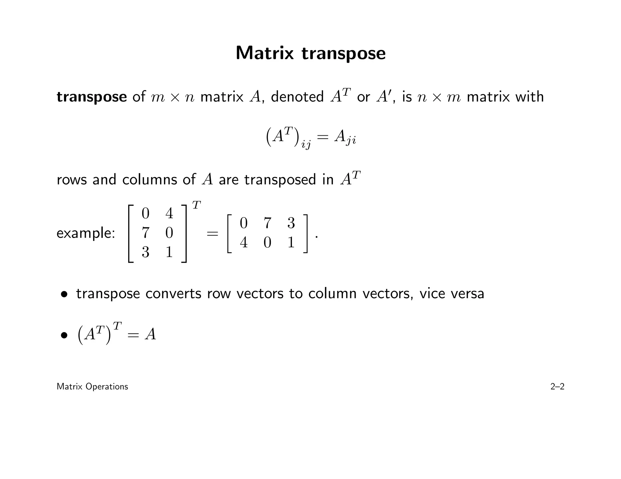
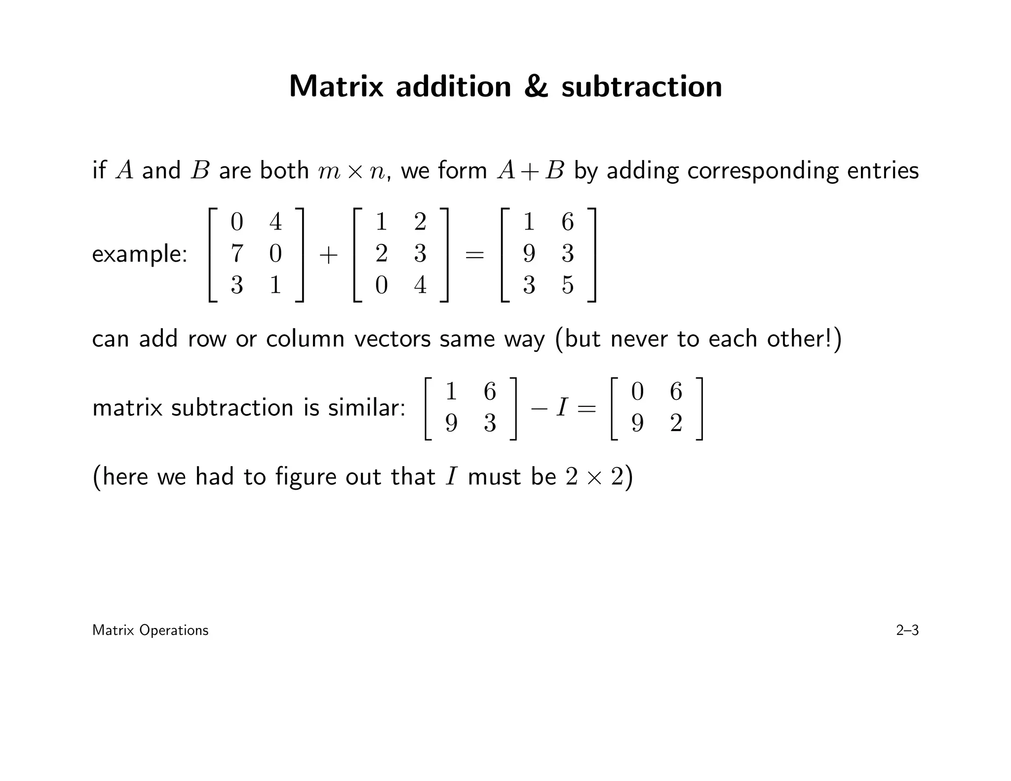
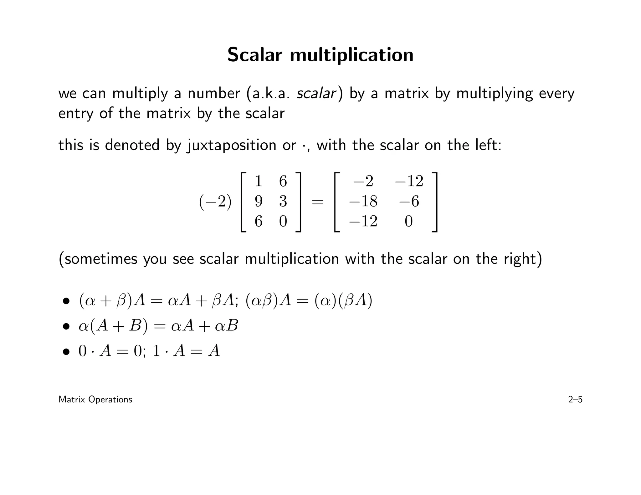
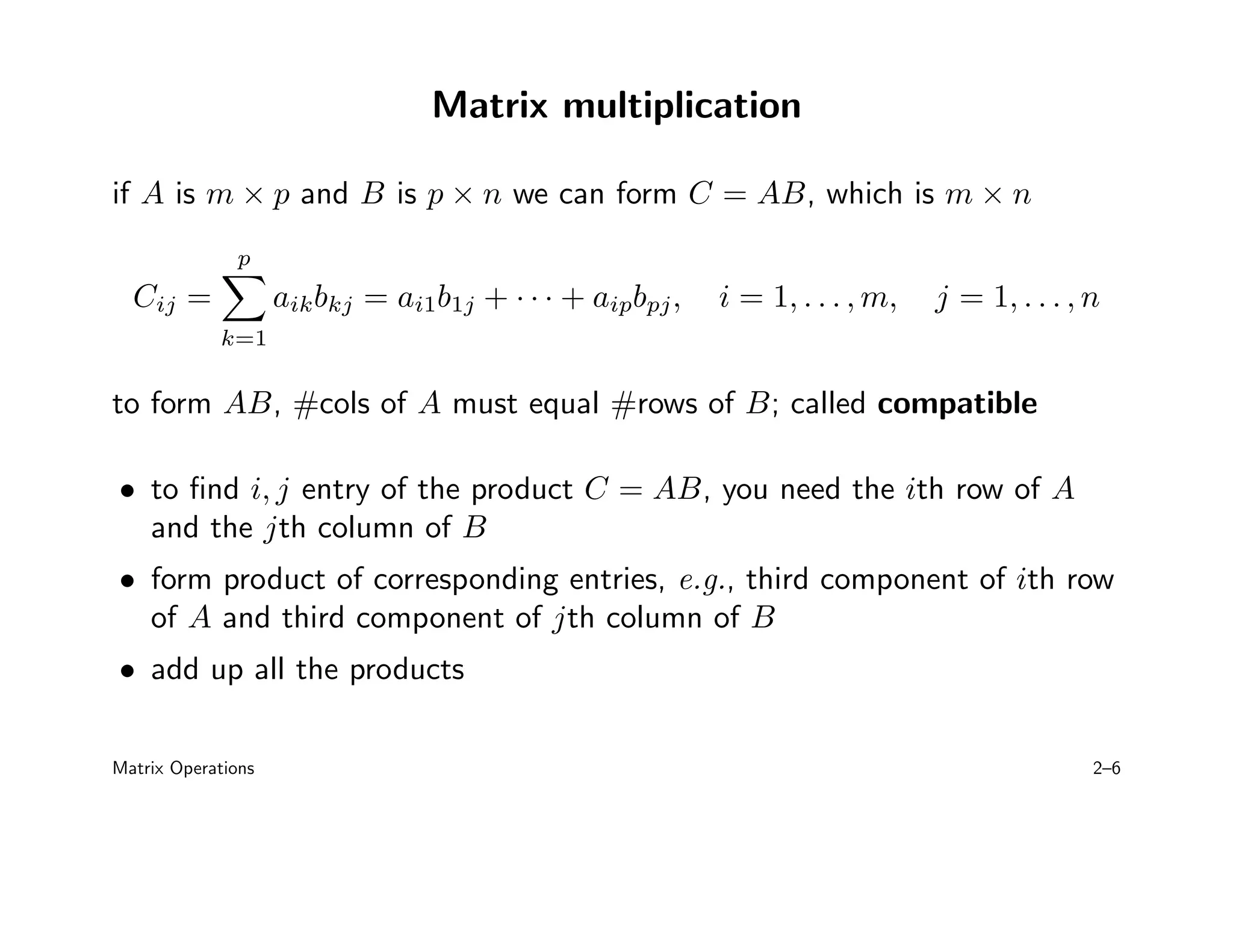
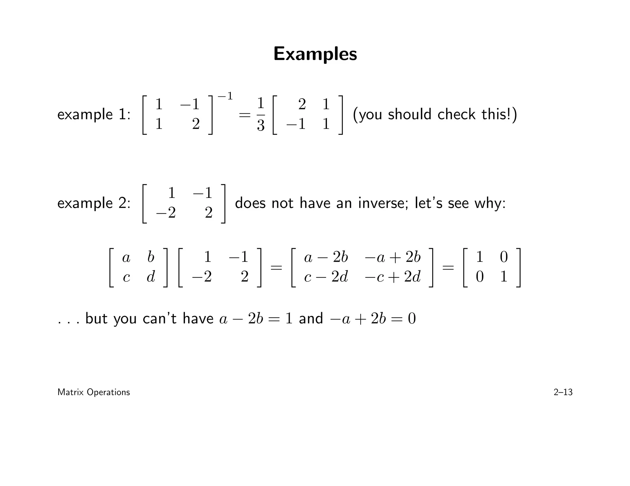
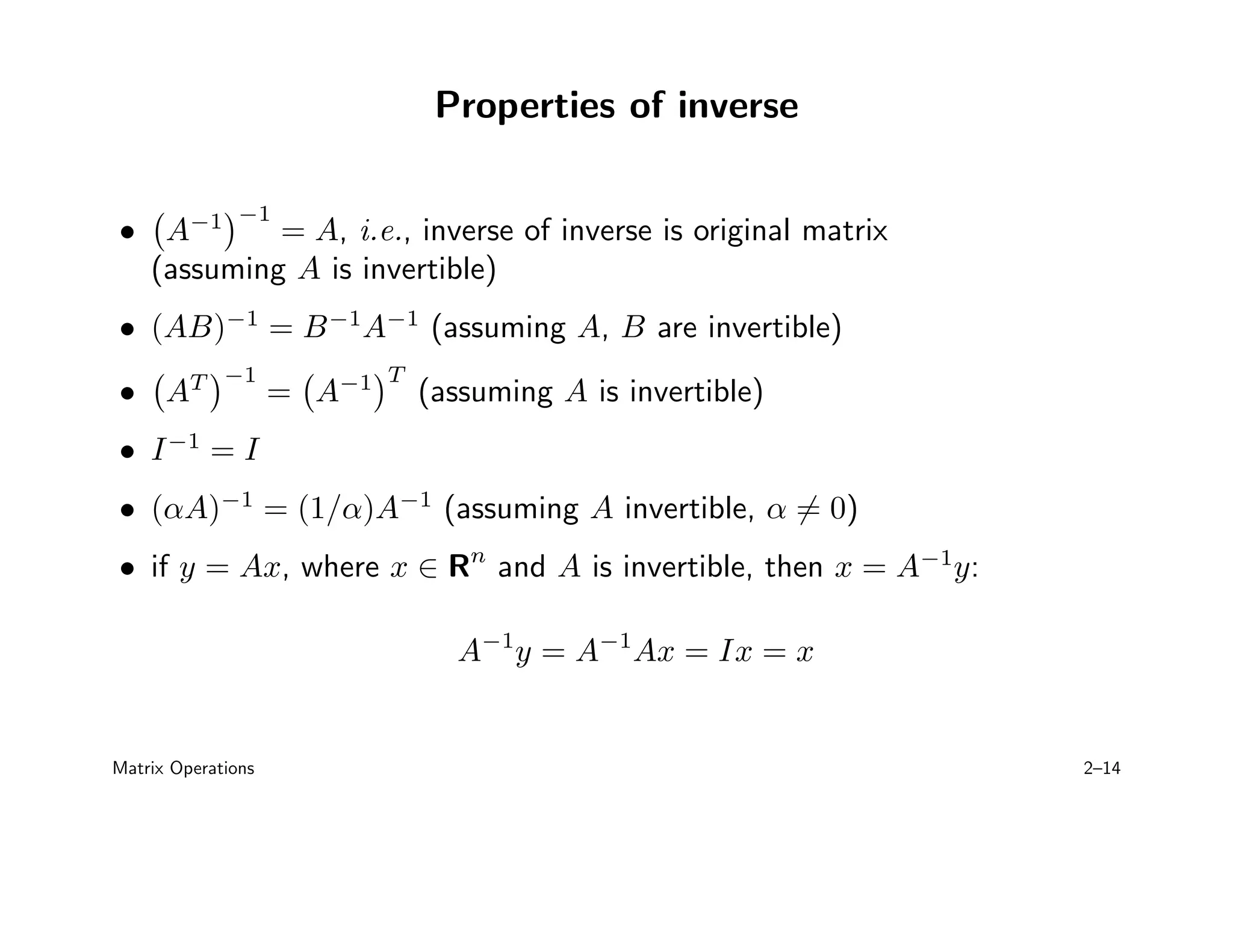
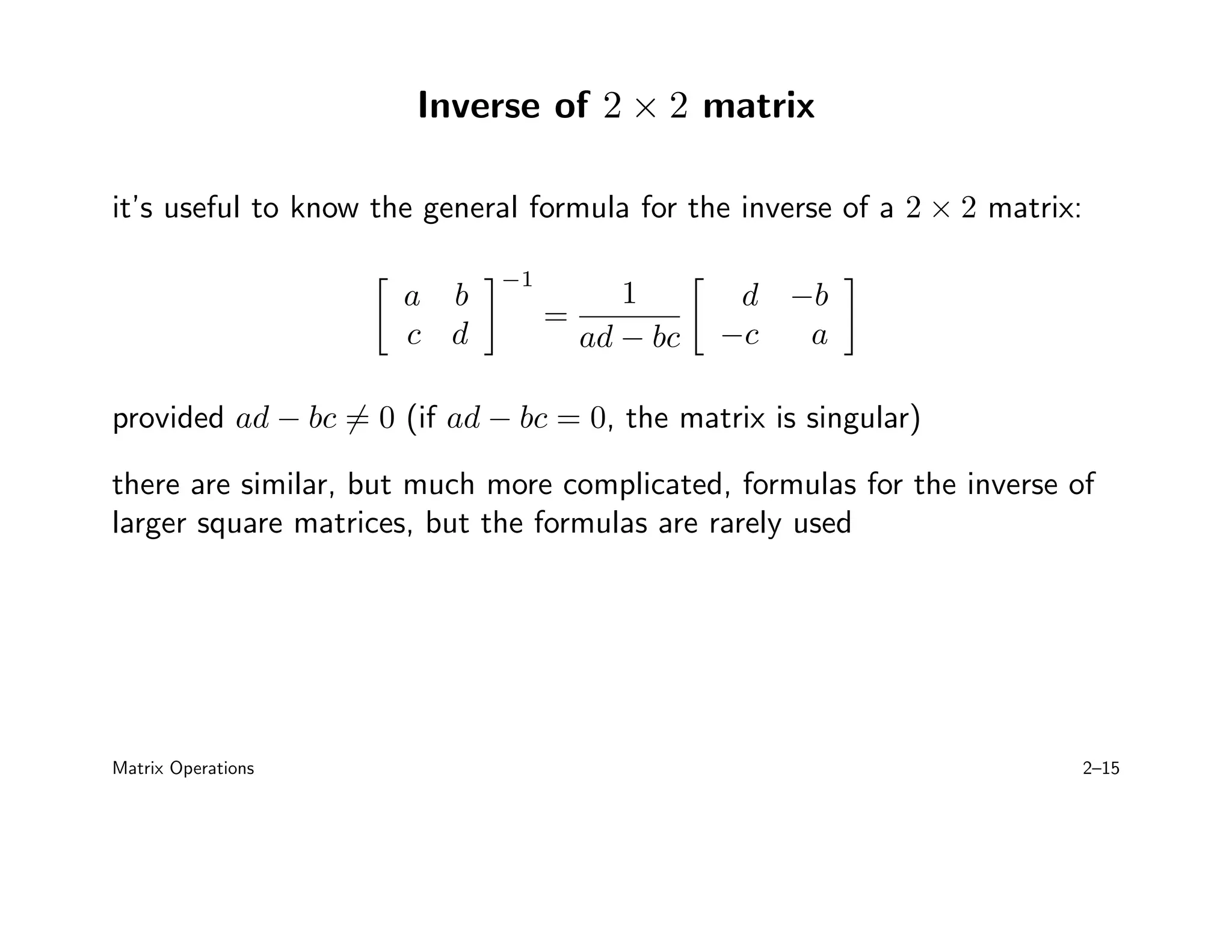
- The document discusses various matrix operations including transpose, addition, subtraction, scalar multiplication, matrix multiplication, matrix-vector products, and finding the inverse of a matrix. - Key operations include transposing a matrix, adding and subtracting matrices of the same size, multiplying a matrix by a scalar, multiplying two matrices if they are compatible in size, and taking the inverse of a square matrix if it exists. 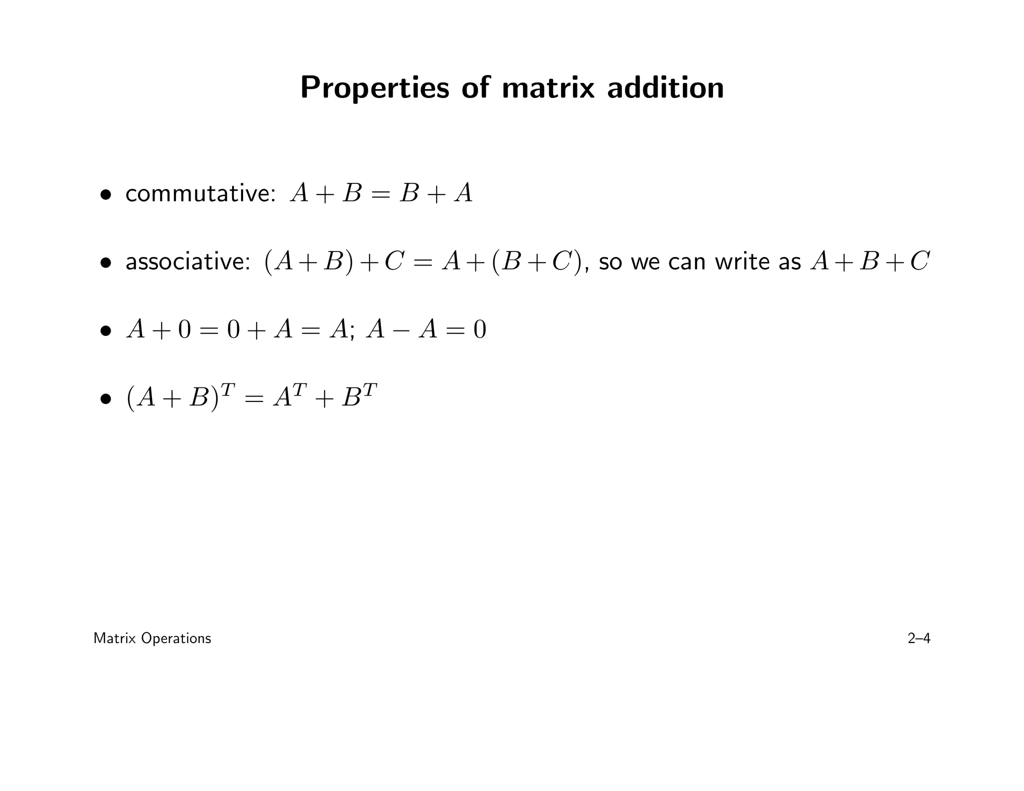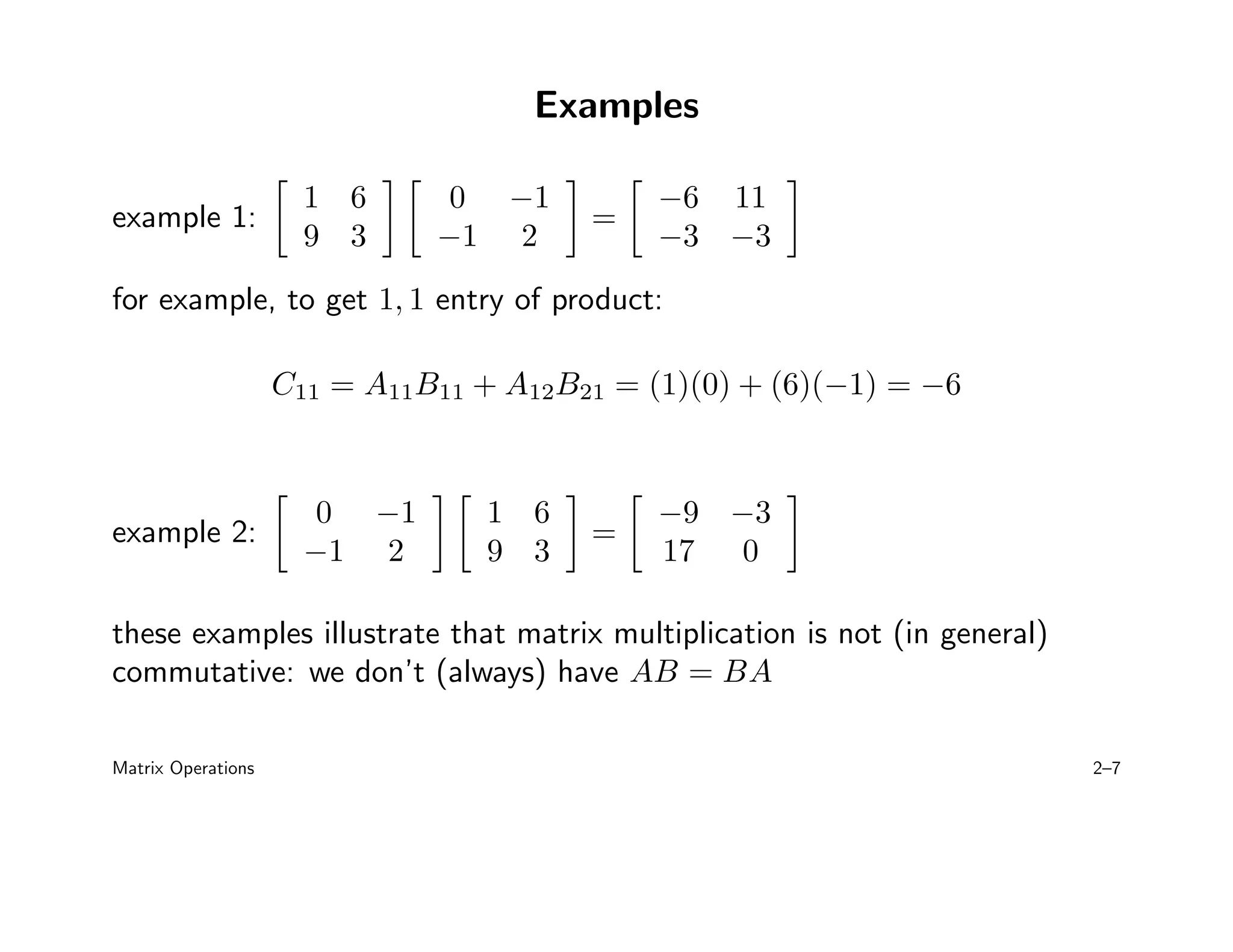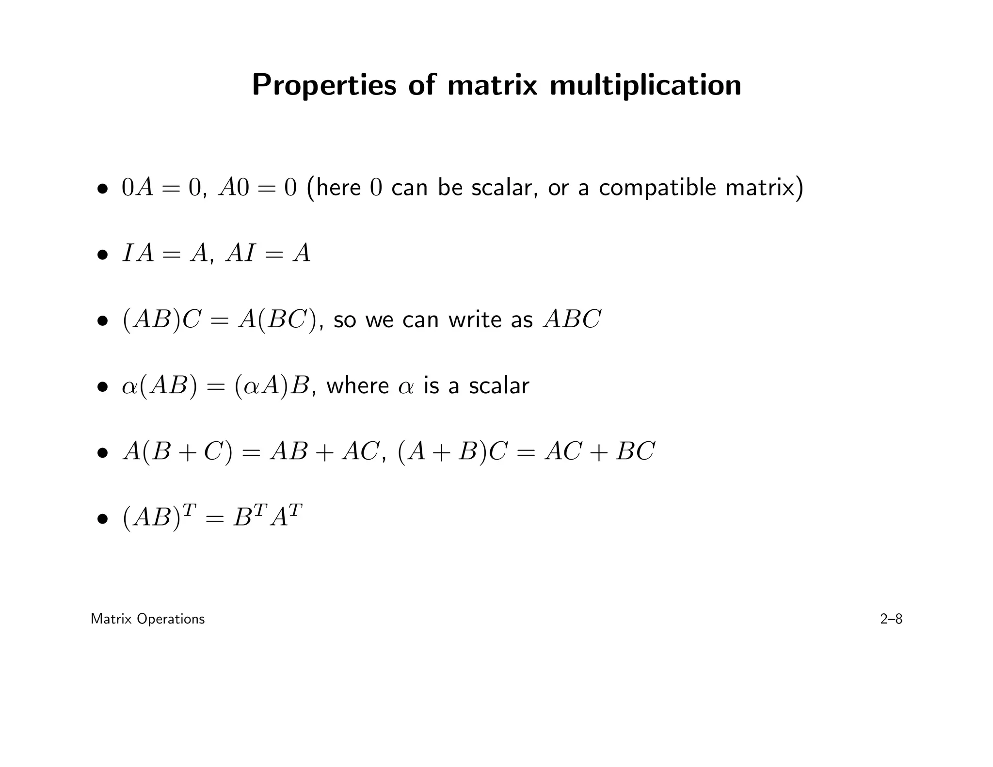- Properties such as commutativity, associativity, and how they apply to different matrix operations are also covered.

1. Lecture 2
Matrix Operations
• transpose, sum & difference, scalar multiplication
• matrix multiplication, matrix-vector product
• matrix inverse
2–1

2. Matrix transpose
transpose of m × n matrix A, denoted AT
or A′
, is n × m matrix with
AT
ij
= Aji
rows and columns of A are transposed in AT
example:


0 4
7 0
3 1


T
=
0 7 3
4 0 1
.
• transpose converts row vectors to column vectors, vice versa
• AT
T
= A
Matrix Operations 2–2

3. Matrix addition subtraction
if A and B are both m × n, we form A + B by adding corresponding entries
example:


0 4
7 0
3 1

 +


1 2
2 3
0 4

 =


1 6
9 3
3 5


can add row or column vectors same way (but never to each other!)
matrix subtraction is similar:
1 6
9 3
− I =
0 6
9 2
(here we had to figure out that I must be 2 × 2)
Matrix Operations 2–3

4. Properties of matrix addition
• commutative: A + B = B + A
• associative: (A + B) + C = A + (B + C), so we can write as A + B + C
• A + 0 = 0 + A = A; A − A = 0
• (A + B)T
= AT
+ BT
Matrix Operations 2–4

5. Scalar multiplication
we can multiply a number (a.k.a. scalar) by a matrix by multiplying every
entry of the matrix by the scalar
this is denoted by juxtaposition or ·, with the scalar on the left:
(−2)


1 6
9 3
6 0

 =


−2 −12
−18 −6
−12 0


(sometimes you see scalar multiplication with the scalar on the right)
• (α + β)A = αA + βA; (αβ)A = (α)(βA)
• α(A + B) = αA + αB
• 0 · A = 0; 1 · A = A
Matrix Operations 2–5

6. Matrix multiplication
if A is m × p and B is p × n we can form C = AB, which is m × n
Cij =
p
X
k=1
aikbkj = ai1b1j + · · · + aipbpj, i = 1, . . . , m, j = 1, . . . , n
to form AB, #cols of A must equal #rows of B; called compatible
• to find i, j entry of the product C = AB, you need the ith row of A
and the jth column of B
• form product of corresponding entries, e.g., third component of ith row
of A and third component of jth column of B
• add up all the products
Matrix Operations 2–6

7. Examples
example 1:
1 6
9 3
0 −1
−1 2
=
−6 11
−3 −3
for example, to get 1, 1 entry of product:
C11 = A11B11 + A12B21 = (1)(0) + (6)(−1) = −6
example 2:
0 −1
−1 2
1 6
9 3
=
−9 −3
17 0
these examples illustrate that matrix multiplication is not (in general)
commutative: we don’t (always) have AB = BA
Matrix Operations 2–7

8. Properties of matrix multiplication
• 0A = 0, A0 = 0 (here 0 can be scalar, or a compatible matrix)
• IA = A, AI = A
• (AB)C = A(BC), so we can write as ABC
• α(AB) = (αA)B, where α is a scalar
• A(B + C) = AB + AC, (A + B)C = AC + BC
• (AB)T
= BT
AT
Matrix Operations 2–8

9. Matrix-vector product
very important special case of matrix multiplication: y = Ax
• A is an m × n matrix
• x is an n-vector
• y is an m-vector
yi = Ai1x1 + · · · + Ainxn, i = 1, . . . , m
can think of y = Ax as
• a function that transforms n-vectors into m-vectors
• a set of m linear equations relating x to y
Matrix Operations 2–9

10. Inner product
if v is a row n-vector and w is a column n-vector, then vw makes sense,
and has size 1 × 1, i.e., is a scalar:
vw = v1w1 + · · · + vnwn
if x and y are n-vectors, xT
y is a scalar called inner product or dot
product of x, y, and denoted hx, yi or x · y:
hx, yi = xT
y = x1y1 + · · · + xnyn
(the symbol · can be ambiguous — it can mean dot product, or ordinary
matrix product)
Matrix Operations 2–10

11. Matrix powers
if matrix A is square, then product AA makes sense, and is denoted A2
more generally, k copies of A multiplied together gives Ak
:
Ak
= A A · · · A
| {z }
k
by convention we set A0
= I
(non-integer powers like A1/2
are tricky — that’s an advanced topic)
we have Ak
Al
= Ak+l
Matrix Operations 2–11

12. Matrix inverse
if A is square, and (square) matrix F satisfies FA = I, then
• F is called the inverse of A, and is denoted A−1
• the matrix A is called invertible or nonsingular
if A doesn’t have an inverse, it’s called singular or noninvertible
by definition, A−1
A = I; a basic result of linear algebra is that AA−1
= I
we define negative powers of A via A−k
= A−1
k
Matrix Operations 2–12

13. Examples
example 1:
1 −1
1 2
−1
=
1
3
2 1
−1 1
(you should check this!)
example 2:
1 −1
−2 2
does not have an inverse; let’s see why:
a b
c d
1 −1
−2 2
=
a − 2b −a + 2b
c − 2d −c + 2d
=
1 0
0 1
. . . but you can’t have a − 2b = 1 and −a + 2b = 0
Matrix Operations 2–13

14. Properties of inverse
• A−1
−1
= A, i.e., inverse of inverse is original matrix
(assuming A is invertible)
• (AB)−1
= B−1
A−1
(assuming A, B are invertible)
• AT
−1
= A−1
T
(assuming A is invertible)
• I−1
= I
• (αA)−1
= (1/α)A−1
(assuming A invertible, α 6= 0)
• if y = Ax, where x ∈ Rn
and A is invertible, then x = A−1
y:
A−1
y = A−1
Ax = Ix = x
Matrix Operations 2–14

15. Inverse of 2 × 2 matrix
it’s useful to know the general formula for the inverse of a 2 × 2 matrix:
a b
c d
−1
=
1
ad − bc
d −b
−c a
provided ad − bc 6= 0 (if ad − bc = 0, the matrix is singular)
there are similar, but much more complicated, formulas for the inverse of
larger square matrices, but the formulas are rarely used
Matrix Operations 2–15