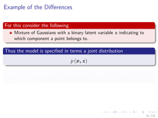
Download as PDF, PPTX


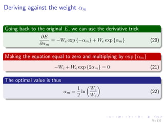
![Images/cinvestav-
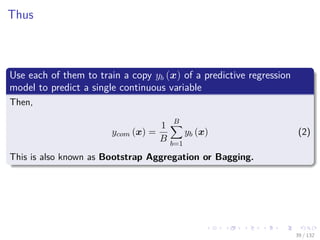
We could use simple averaging
Given a series of observed samples {x1, x2, ..., xN } with noise
∼ N (0, 1)
We could use our knowledge on the noise, for example additive:
xi = xi +
We can use our knowledge of probability to remove such noise
E [xi] = E [xi + ] = E [xi] + E [ ]
Then, because E [ ] = 0
E [xi] = E [xi] ≈
1
N
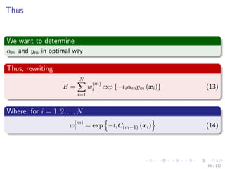
N
i=1
xi
6 / 132](https://image.slidesharecdn.com/18-180731144505/85/18-1-combining-models-10-320.jpg)
![Images/cinvestav-
We could use simple averaging
Given a series of observed samples {x1, x2, ..., xN } with noise
∼ N (0, 1)
We could use our knowledge on the noise, for example additive:
xi = xi +
We can use our knowledge of probability to remove such noise
E [xi] = E [xi + ] = E [xi] + E [ ]
Then, because E [ ] = 0
E [xi] = E [xi] ≈
1
N
N
i=1
xi
6 / 132](https://image.slidesharecdn.com/18-180731144505/85/18-1-combining-models-11-320.jpg)
![Images/cinvestav-
We could use simple averaging
Given a series of observed samples {x1, x2, ..., xN } with noise
∼ N (0, 1)
We could use our knowledge on the noise, for example additive:
xi = xi +
We can use our knowledge of probability to remove such noise
E [xi] = E [xi + ] = E [xi] + E [ ]
Then, because E [ ] = 0
E [xi] = E [xi] ≈
1
N
N
i=1
xi
6 / 132](https://image.slidesharecdn.com/18-180731144505/85/18-1-combining-models-12-320.jpg)


![Images/cinvestav-
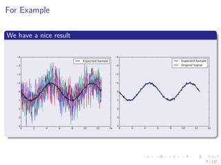
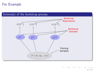
For Example
Its variance
V ar [S (Z)] =
1
B − 1
B
b=1
S Z∗b
− S
∗ 2
Where
S
∗
=
1
B
B
b=1
S Z∗b
35 / 132](https://image.slidesharecdn.com/18-180731144505/85/18-1-combining-models-68-320.jpg)
![Images/cinvestav-
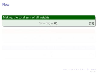
For Example
Its variance
V ar [S (Z)] =
1
B − 1
B
b=1
S Z∗b
− S
∗ 2
Where
S
∗
=
1
B
B
b=1
S Z∗b
35 / 132](https://image.slidesharecdn.com/18-180731144505/85/18-1-combining-models-69-320.jpg)

![Images/cinvestav-
Relation with Monte-Carlo Estimation
Note that V ar [S (Z)]
It can be thought of as a Monte-Carlo estimate of the variance of
S (Z) under sampling.
This is coming
From the empirical distribution function F for the data
Z = {z1, z2, ..., zN }
37 / 132](https://image.slidesharecdn.com/18-180731144505/85/18-1-combining-models-71-320.jpg)
![Images/cinvestav-
Relation with Monte-Carlo Estimation
Note that V ar [S (Z)]
It can be thought of as a Monte-Carlo estimate of the variance of
S (Z) under sampling.
This is coming
From the empirical distribution function F for the data
Z = {z1, z2, ..., zN }
37 / 132](https://image.slidesharecdn.com/18-180731144505/85/18-1-combining-models-72-320.jpg)
![Images/cinvestav-
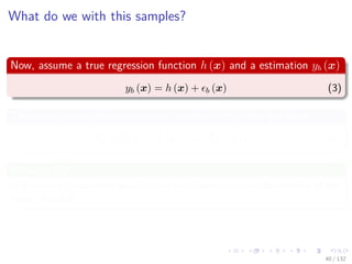
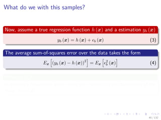
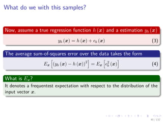
Assume that the errors have zero mean and are
uncorrelated
Assume that the errors have zero mean and are uncorrelated
Something Reasonable to assume given the way we produce the
Bootstrap Samples
Ex [ b (x)] =0
Ex [ b (x) l (x)] = 0, for b = l
42 / 132](https://image.slidesharecdn.com/18-180731144505/85/18-1-combining-models-80-320.jpg)


![Images/cinvestav-
This comes from
The paper
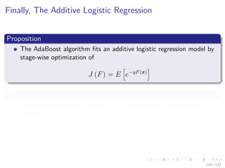
“Additive Logistic Regression: A Statistical View of Boosting” by
Friedman, Hastie and Tibshirani
Something Notable
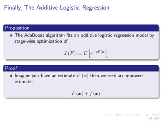
In this paper, a proof exists to show that boosting algorithms are
procedures to fit and additive logistic regression model.
E [y|x] = F (x) with F (x) =
M
m=1
fm (x)
100 / 132](https://image.slidesharecdn.com/18-180731144505/85/18-1-combining-models-215-320.jpg)
![Images/cinvestav-
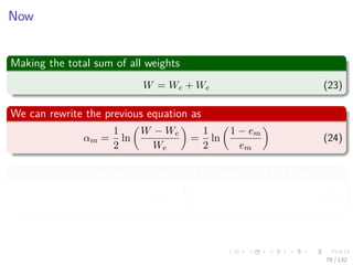
This comes from
The paper
“Additive Logistic Regression: A Statistical View of Boosting” by
Friedman, Hastie and Tibshirani
Something Notable
In this paper, a proof exists to show that boosting algorithms are
procedures to fit and additive logistic regression model.
E [y|x] = F (x) with F (x) =
M
m=1
fm (x)
100 / 132](https://image.slidesharecdn.com/18-180731144505/85/18-1-combining-models-216-320.jpg)
![Images/cinvestav-
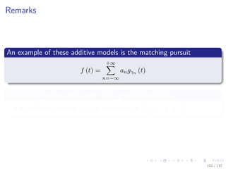
Consider the Additive Regression Model
We are interested in modeling the mean E [y|x] = F (x)
With Additive Model
F (x) =
d
i=1
fi (xi)
Where each fi (xi) is a function for each feature input xi
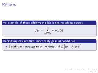
A convenient algorithm for updating these models it the backfitting
algorithm with update:
fi (xi) = E
y −
k=i
fk (xk) |xi
101 / 132](https://image.slidesharecdn.com/18-180731144505/85/18-1-combining-models-217-320.jpg)
![Images/cinvestav-
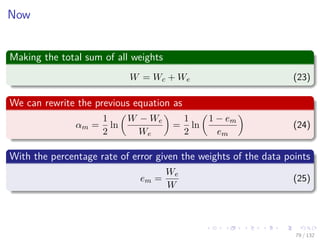
Consider the Additive Regression Model
We are interested in modeling the mean E [y|x] = F (x)
With Additive Model
F (x) =
d
i=1
fi (xi)
Where each fi (xi) is a function for each feature input xi
A convenient algorithm for updating these models it the backfitting
algorithm with update:
fi (xi) = E
y −
k=i
fk (xk) |xi
101 / 132](https://image.slidesharecdn.com/18-180731144505/85/18-1-combining-models-218-320.jpg)
![Images/cinvestav-
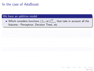
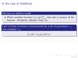
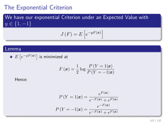
Remark - Moving from Regression to Classification
Given that Regression have wide ranges of outputs
Logistic Regression is widely used to move Regression to Classification
log
P (Y = 1|x)
P (Y = −1|x)
=
M
m=1
fm (x)
A nice property, the probability estimates lie in [0, 1]
Now, solving by assuming P (Y = 1|x) + P (Y = −1|x) = 1
P (Y = 1|x) =
eF(x)
1 + eF(x)
105 / 132](https://image.slidesharecdn.com/18-180731144505/85/18-1-combining-models-225-320.jpg)
![Images/cinvestav-
Remark - Moving from Regression to Classification
Given that Regression have wide ranges of outputs
Logistic Regression is widely used to move Regression to Classification
log
P (Y = 1|x)
P (Y = −1|x)
=
M
m=1
fm (x)
A nice property, the probability estimates lie in [0, 1]
Now, solving by assuming P (Y = 1|x) + P (Y = −1|x) = 1
P (Y = 1|x) =
eF(x)
1 + eF(x)
105 / 132](https://image.slidesharecdn.com/18-180731144505/85/18-1-combining-models-226-320.jpg)
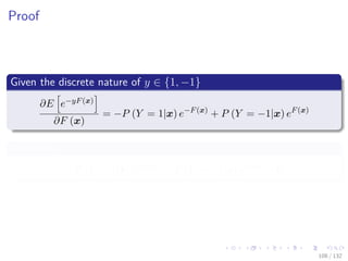
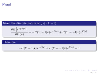
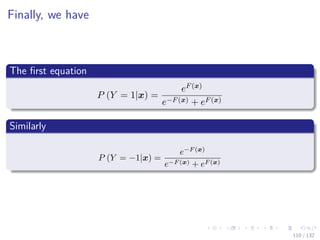
![Images/cinvestav-
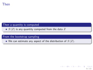
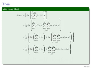
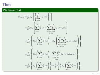
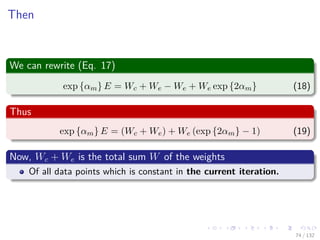
Then
We have that
P (Y = 1|x) e−F(x)
= P (Y = −1|x) eF(x)
= [1 − P (Y = 1|x)] eF(x)
Solving
eF(x)
= e−F(x)
+ eF(x)
P (Y = 1|x)
109 / 132](https://image.slidesharecdn.com/18-180731144505/85/18-1-combining-models-232-320.jpg)
![Images/cinvestav-
Then
We have that
P (Y = 1|x) e−F(x)
= P (Y = −1|x) eF(x)
= [1 − P (Y = 1|x)] eF(x)
Solving
eF(x)
= e−F(x)
+ eF(x)
P (Y = 1|x)
109 / 132](https://image.slidesharecdn.com/18-180731144505/85/18-1-combining-models-233-320.jpg)


![Images/cinvestav-
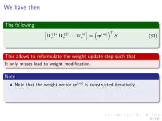
We have the following
If we divide by E e−yF(x)
|x , the first term
E e−yF (x)
I (y = 1) |x
E [e−yF (x)|x]
= Ew [I (y = 1) |x]
Also
E e−yF (x)
I (y = −1) |x
E [e−yF (x)|x]
= Ew [I (y = −1) |x]
117 / 132](https://image.slidesharecdn.com/18-180731144505/85/18-1-combining-models-246-320.jpg)
![Images/cinvestav-
We have the following
If we divide by E e−yF(x)
|x , the first term
E e−yF (x)
I (y = 1) |x
E [e−yF (x)|x]
= Ew [I (y = 1) |x]
Also
E e−yF (x)
I (y = −1) |x
E [e−yF (x)|x]
= Ew [I (y = −1) |x]
117 / 132](https://image.slidesharecdn.com/18-180731144505/85/18-1-combining-models-247-320.jpg)
![Images/cinvestav-
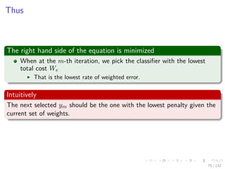
Thus, we have
We apply the natural log to both sides
log e−f(x)
+ log Ew [I (y = 1) |x] = log ef(x)
+ log Ew [I (y = −1) |x]
Then
2f (x) = log Ew [I (y = 1) |x] − log Ew [I (y = −1) |x]
118 / 132](https://image.slidesharecdn.com/18-180731144505/85/18-1-combining-models-248-320.jpg)
![Images/cinvestav-
Thus, we have
We apply the natural log to both sides
log e−f(x)
+ log Ew [I (y = 1) |x] = log ef(x)
+ log Ew [I (y = −1) |x]
Then
2f (x) = log Ew [I (y = 1) |x] − log Ew [I (y = −1) |x]
118 / 132](https://image.slidesharecdn.com/18-180731144505/85/18-1-combining-models-249-320.jpg)
![Images/cinvestav-
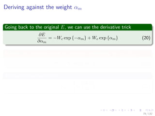
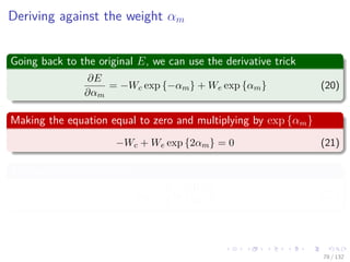
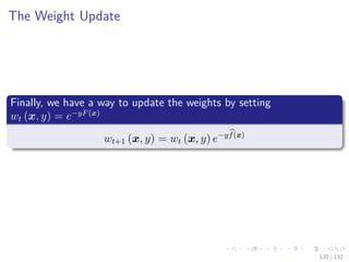
Finally
We have that
f (x) =
1
2
log
Ew [I (y = 1) |x]
Ew [I (y = −1) |x]
In term of probabilities
f (x) =
1
2
log
Pw (y = 1|x)
Pw (y = −1|x)
119 / 132](https://image.slidesharecdn.com/18-180731144505/85/18-1-combining-models-250-320.jpg)
![Images/cinvestav-
Finally
We have that
f (x) =
1
2
log
Ew [I (y = 1) |x]
Ew [I (y = −1) |x]
In term of probabilities
f (x) =
1
2
log
Pw (y = 1|x)
Pw (y = −1|x)
119 / 132](https://image.slidesharecdn.com/18-180731144505/85/18-1-combining-models-251-320.jpg)


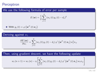
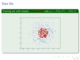
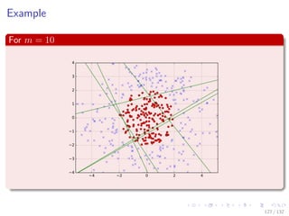
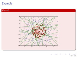

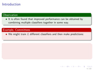
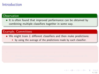
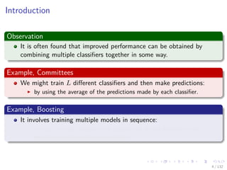
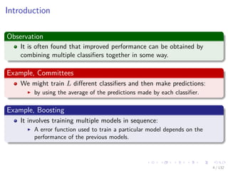
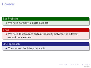
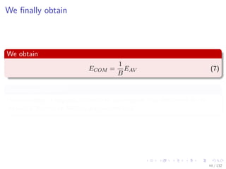
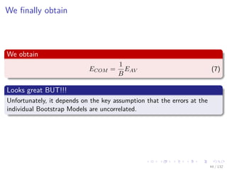
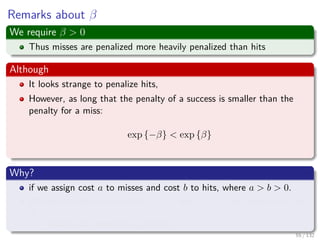
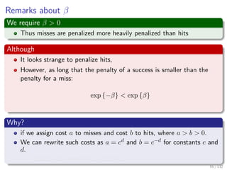
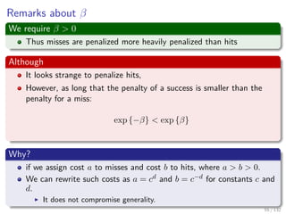
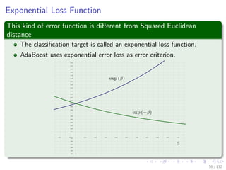
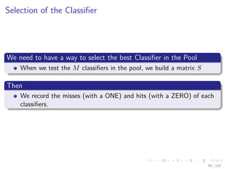
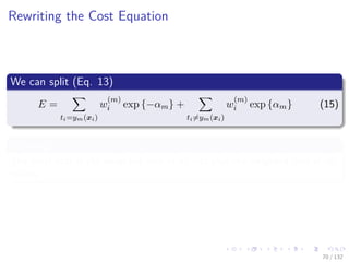
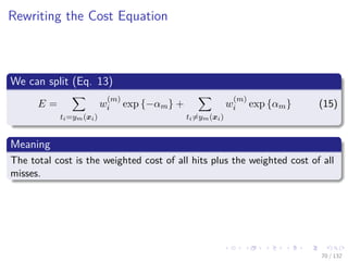
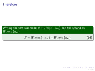
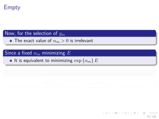
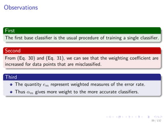
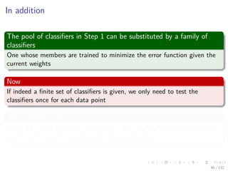
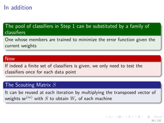
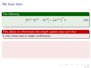
The document provides an introduction to machine learning techniques involving model combinations, Bayesian model averaging, and boosting. It discusses the benefits of combining multiple classifiers, including through committees and sequential training, and differentiates between various averaging methods. Furthermore, it outlines the workings of algorithms like AdaBoost and the relation between decision trees and model predictions.