Download as PDF, PPTX


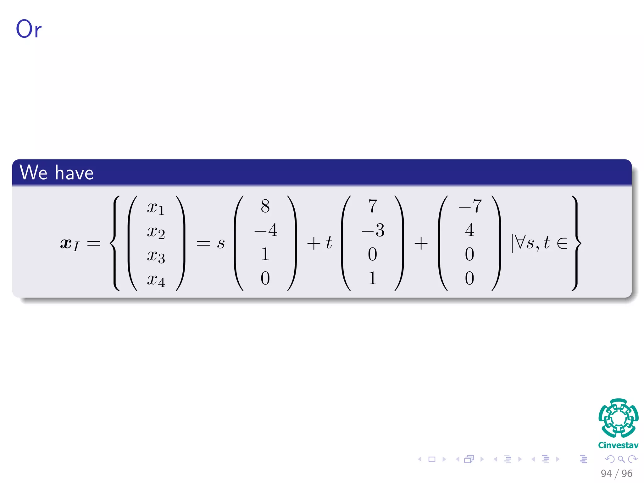
![We have
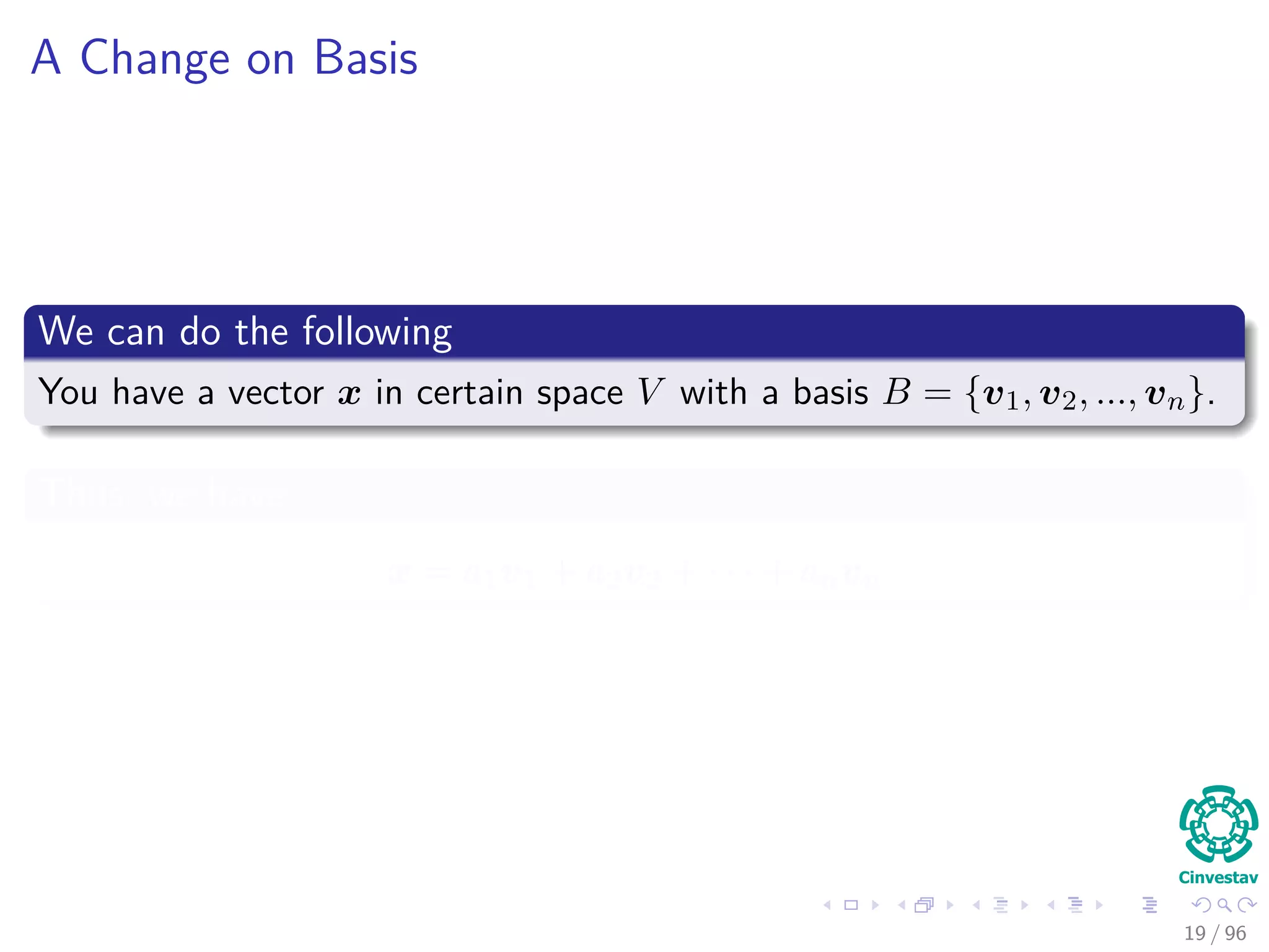
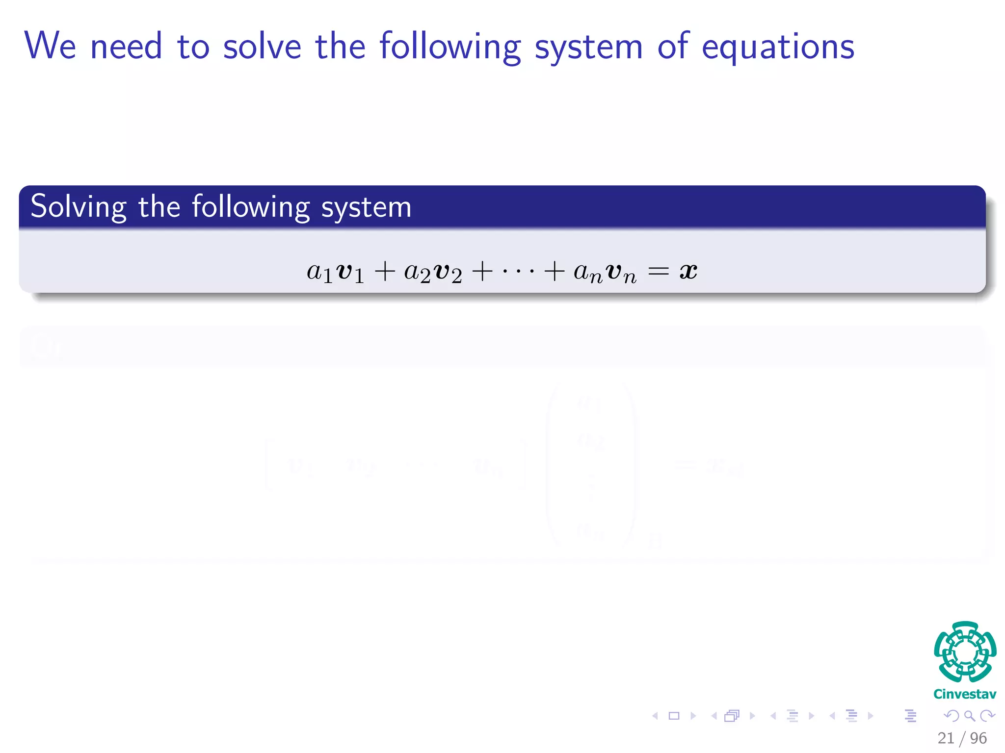
Then in the basis B = {v1, v2, ..., vn}
[x]B =
a1
a2
...
an
B
20 / 96](https://image.slidesharecdn.com/01-200420204420/75/01-02-linear-equations-30-2048.jpg)

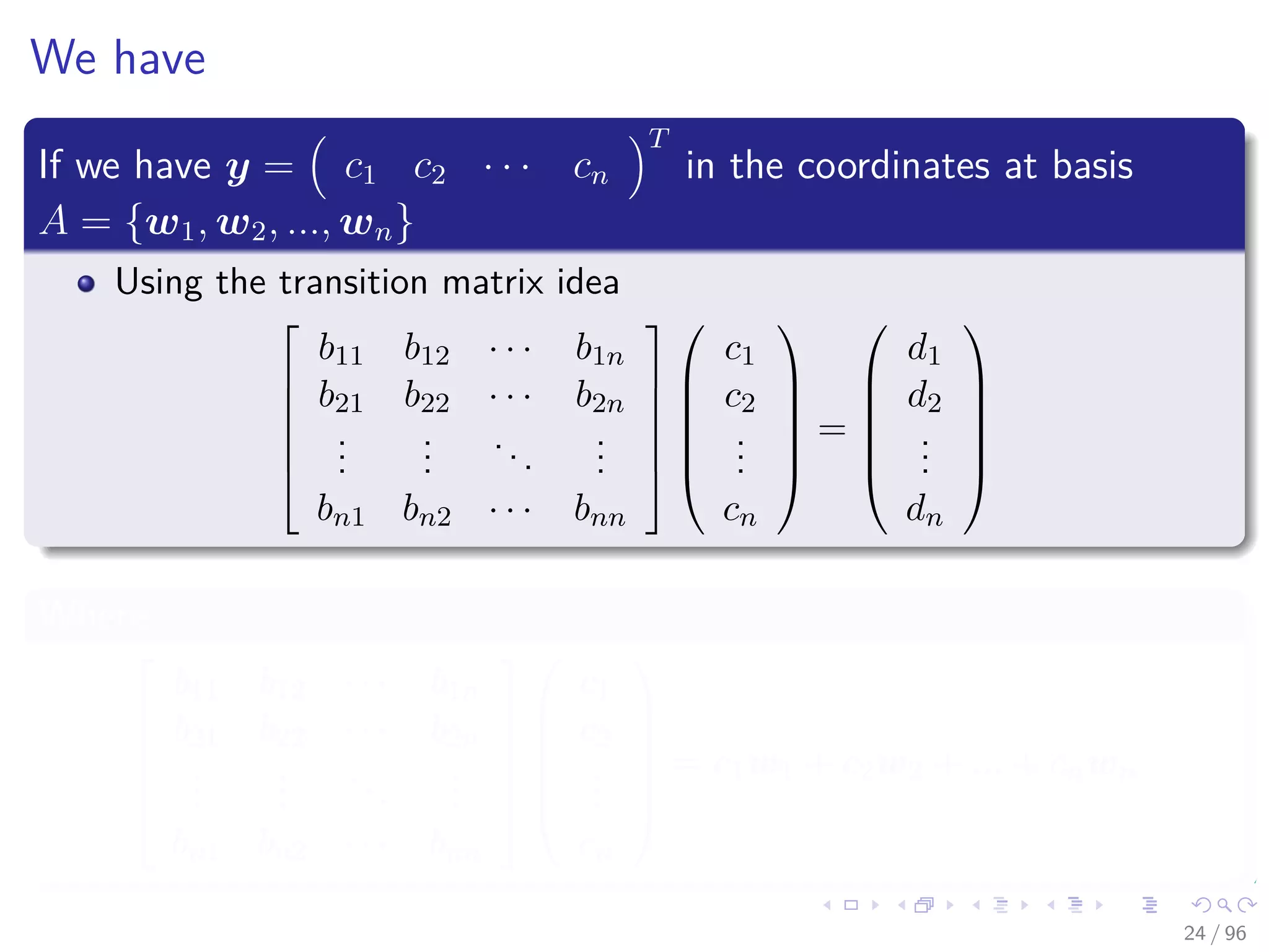
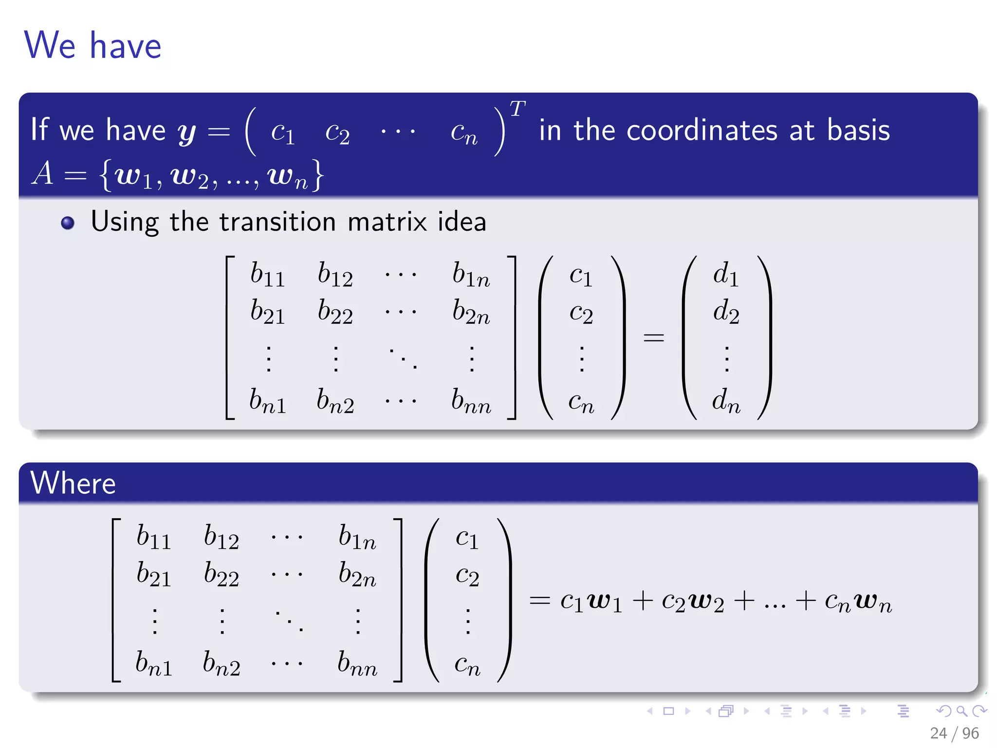
![With the following property
Then using the B = {v1, v2, ..., vn} representation
ciwi = cib1iv1 + cib2iv2 + · · · + cibnivm
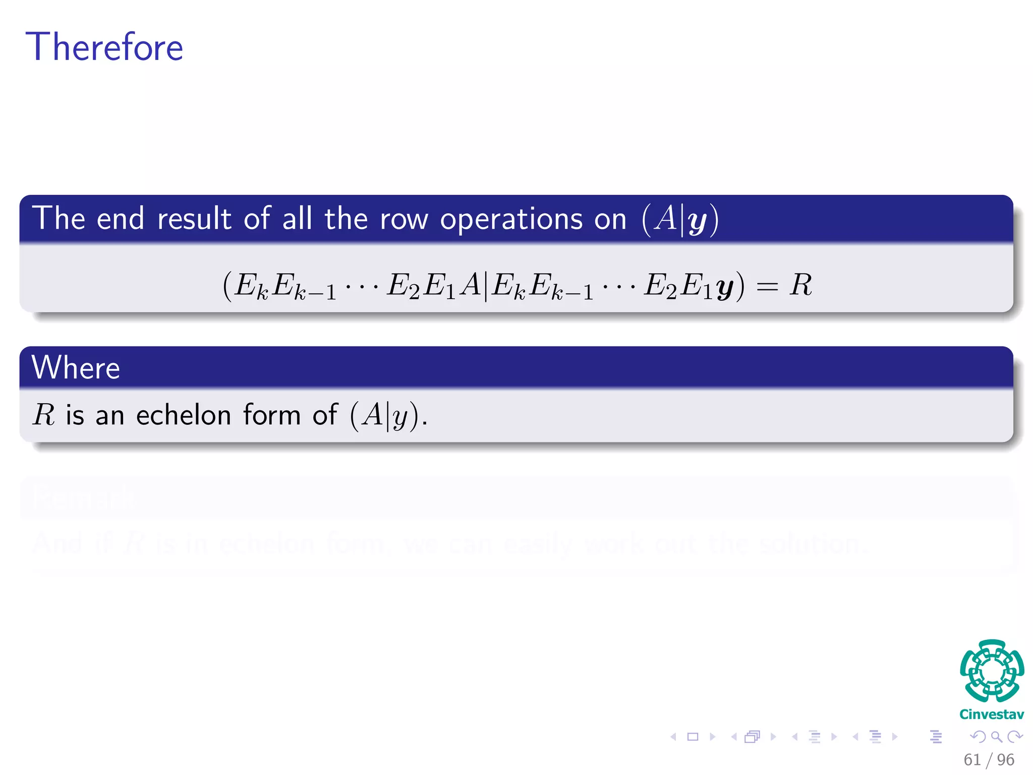
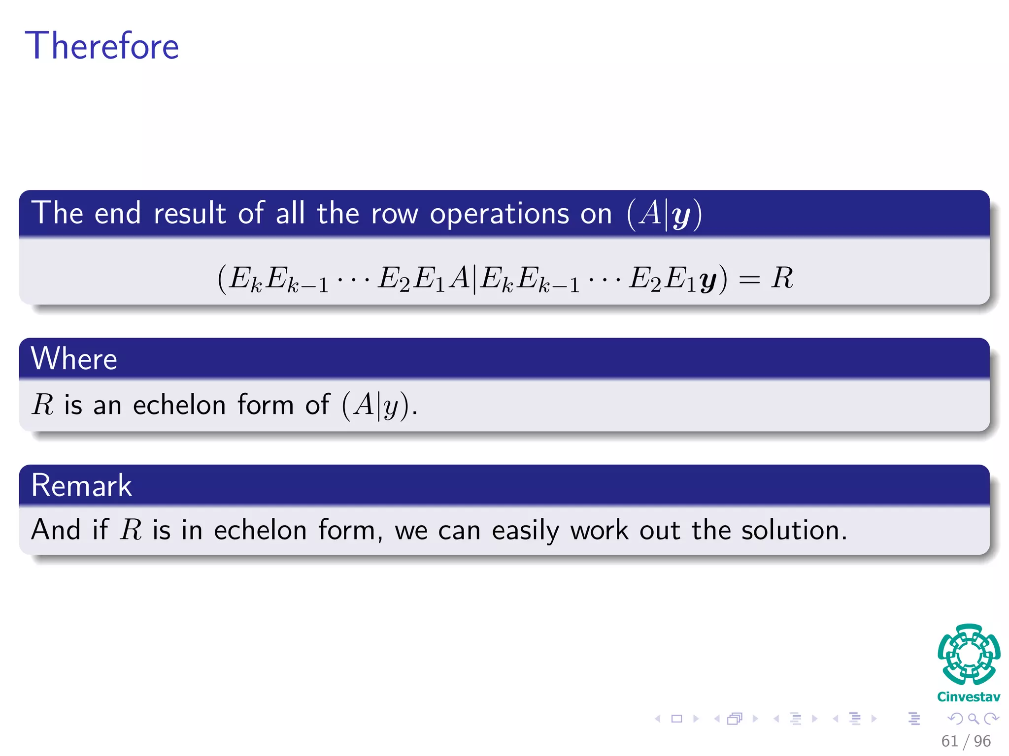
Therefore
(c1b11 + ... + cnb1n) v1 + · · · + (c1bn1 + ... + cnbnn) vn = [x]B
25 / 96](https://image.slidesharecdn.com/01-200420204420/75/01-02-linear-equations-38-2048.jpg)
![With the following property
Then using the B = {v1, v2, ..., vn} representation
ciwi = cib1iv1 + cib2iv2 + · · · + cibnivm
Therefore
(c1b11 + ... + cnb1n) v1 + · · · + (c1bn1 + ... + cnbnn) vn = [x]B
25 / 96](https://image.slidesharecdn.com/01-200420204420/75/01-02-linear-equations-39-2048.jpg)

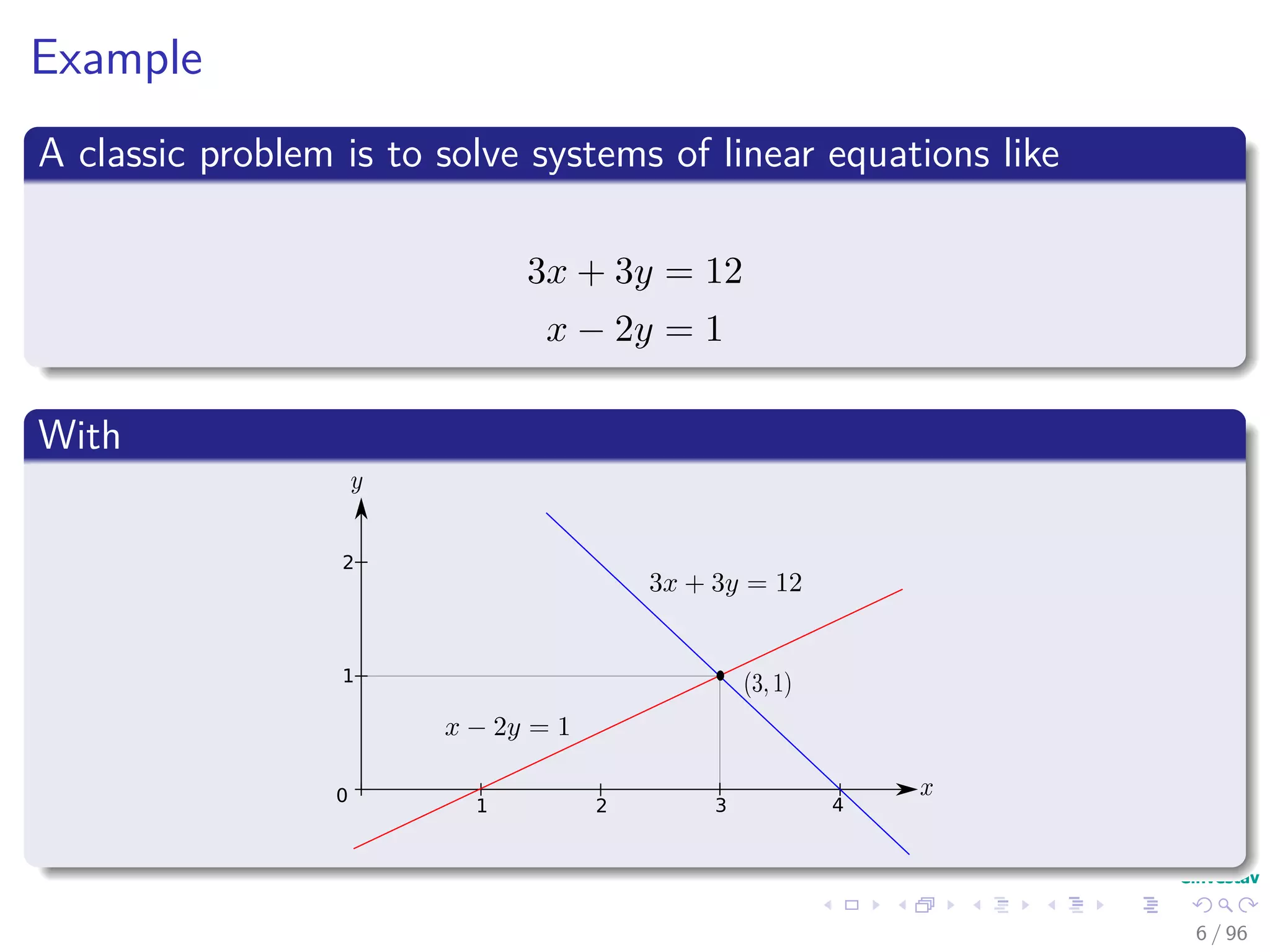
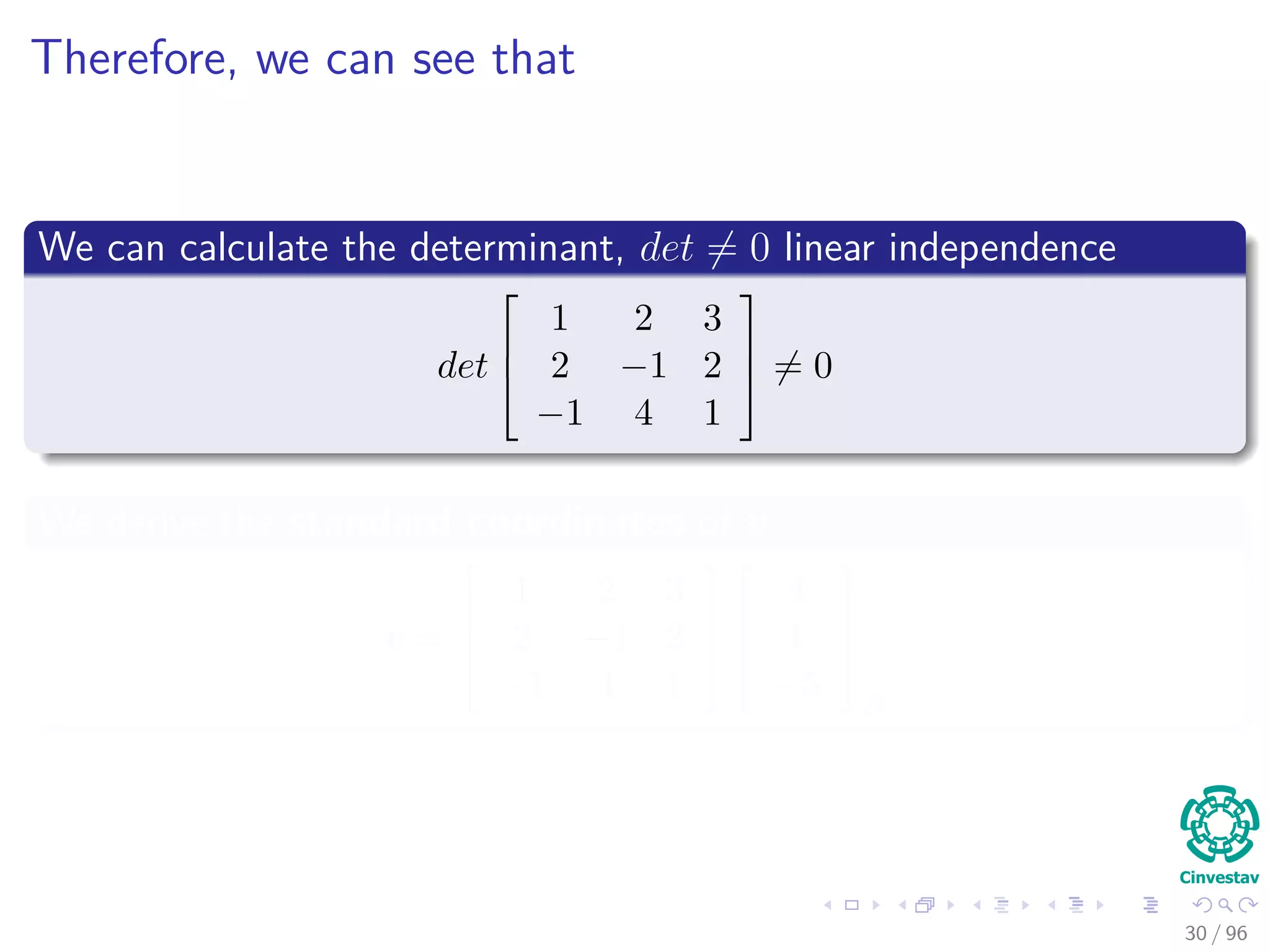
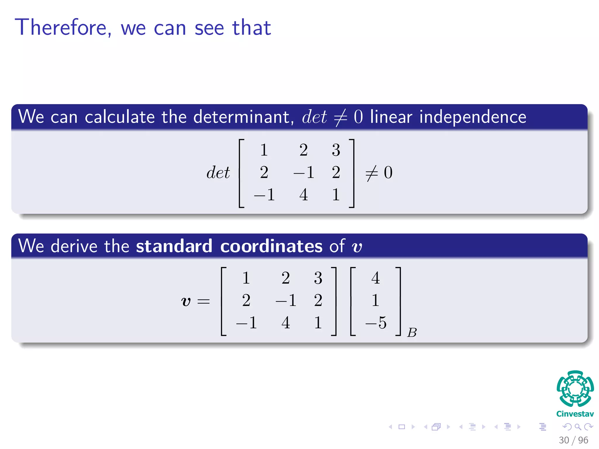
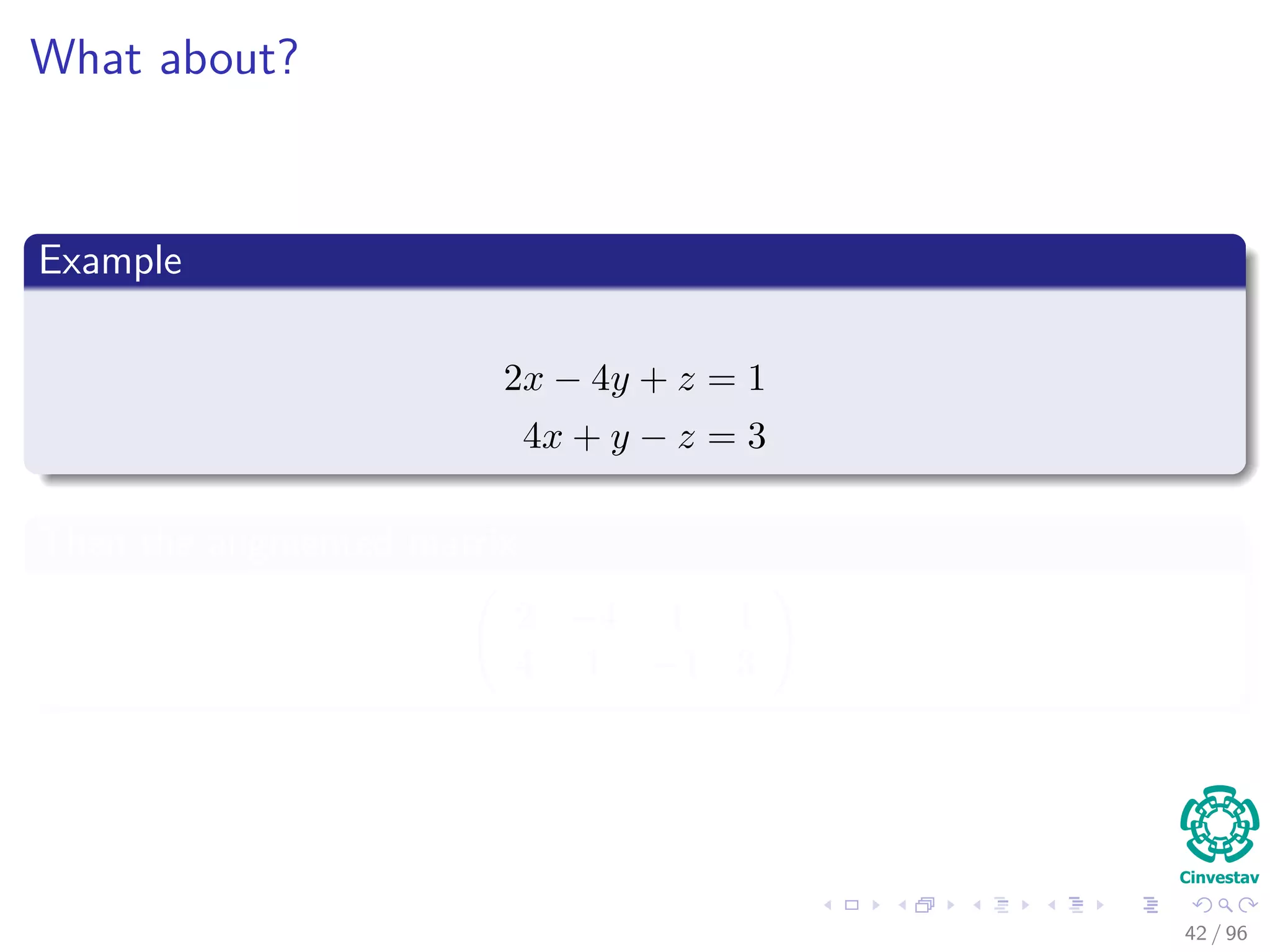
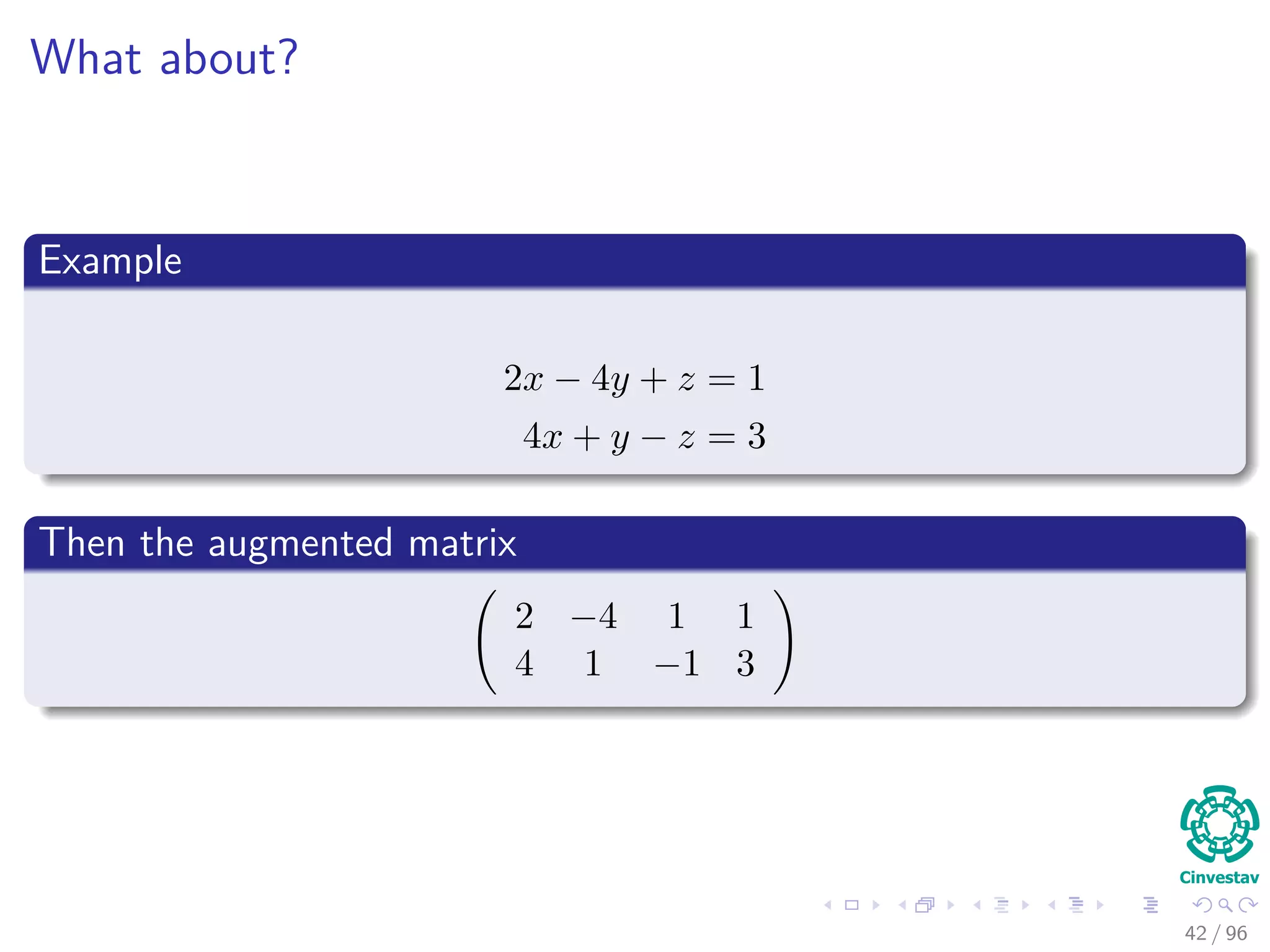
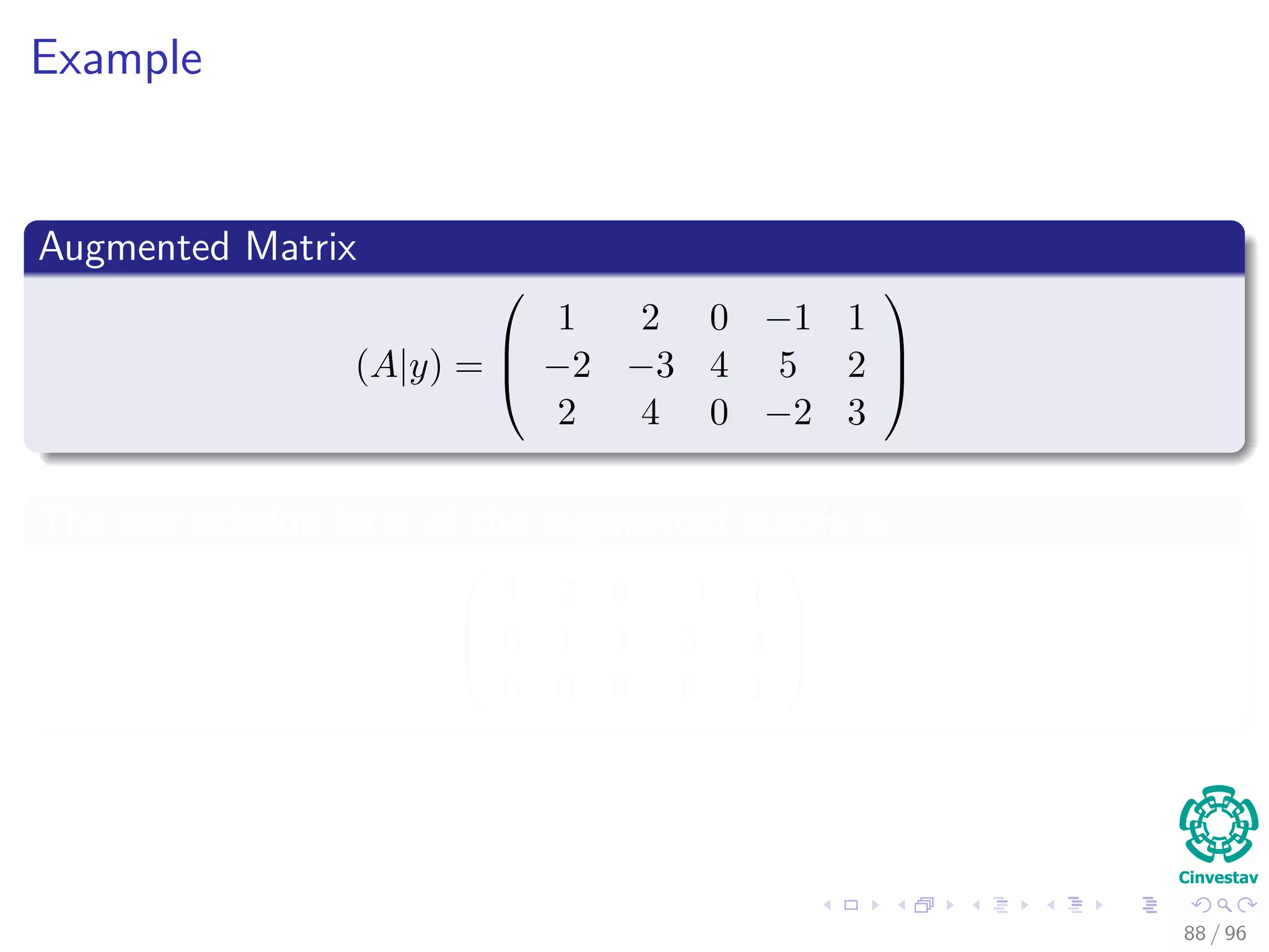
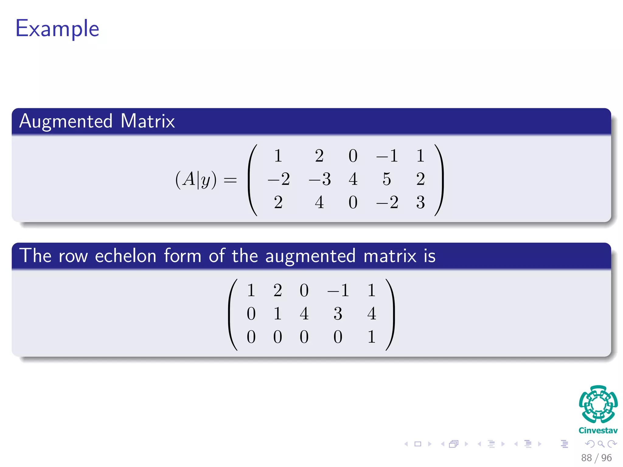
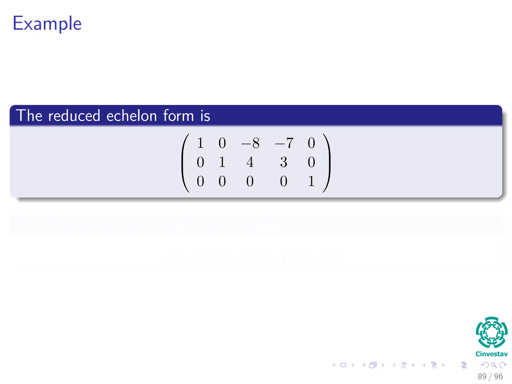
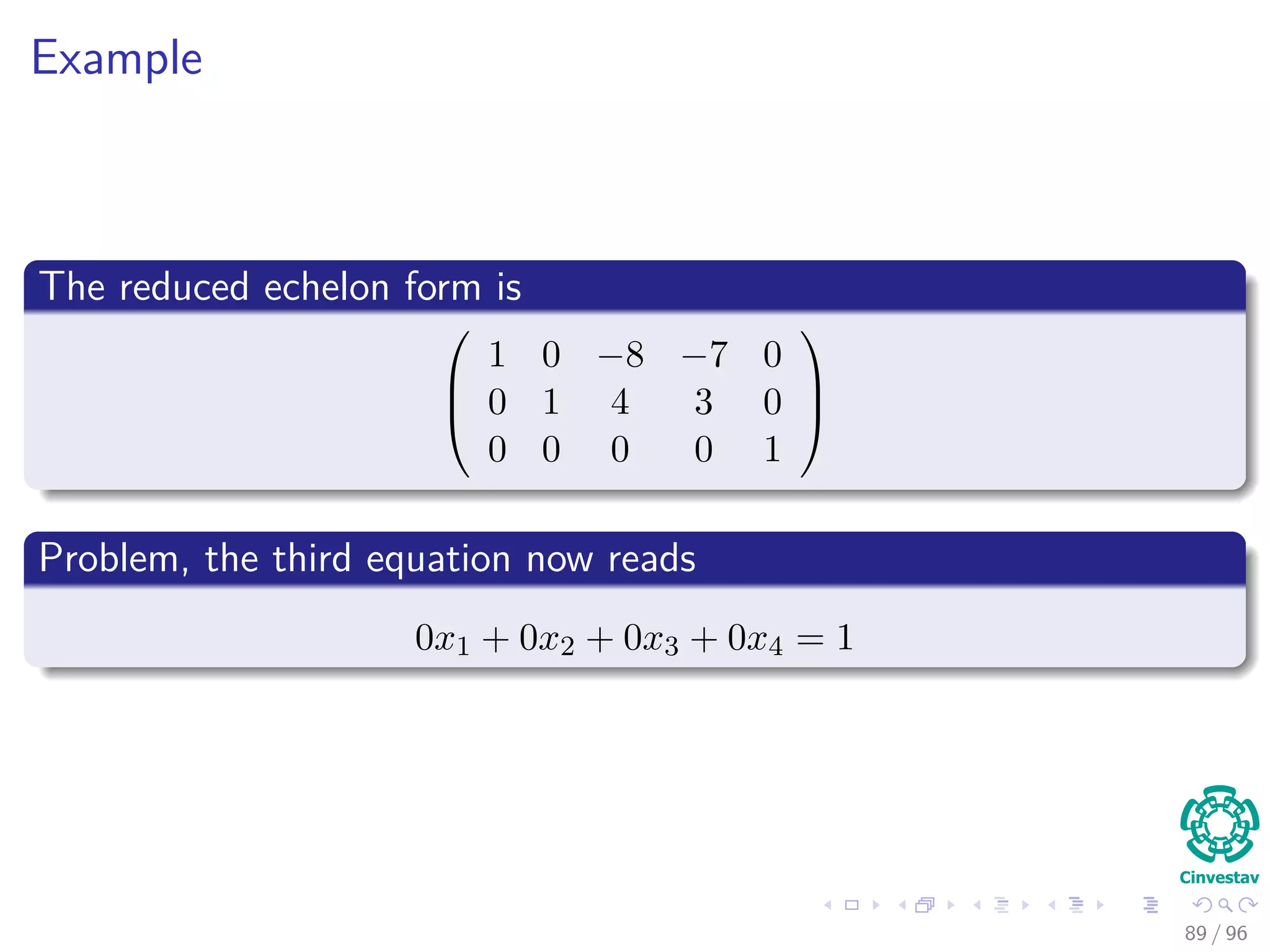
![Example
We have
B =
1
2
−1
,
2
1
4
,
3
2
1
, [v]B =
4
1
−5
B
Transition Matrix
P =
1 2 3
2 −1 2
−1 4 1
29 / 96](https://image.slidesharecdn.com/01-200420204420/75/01-02-linear-equations-45-2048.jpg)
![Example
We have
B =
1
2
−1
,
2
1
4
,
3
2
1
, [v]B =
4
1
−5
B
Transition Matrix
P =
1 2 3
2 −1 2
−1 4 1
29 / 96](https://image.slidesharecdn.com/01-200420204420/75/01-02-linear-equations-46-2048.jpg)
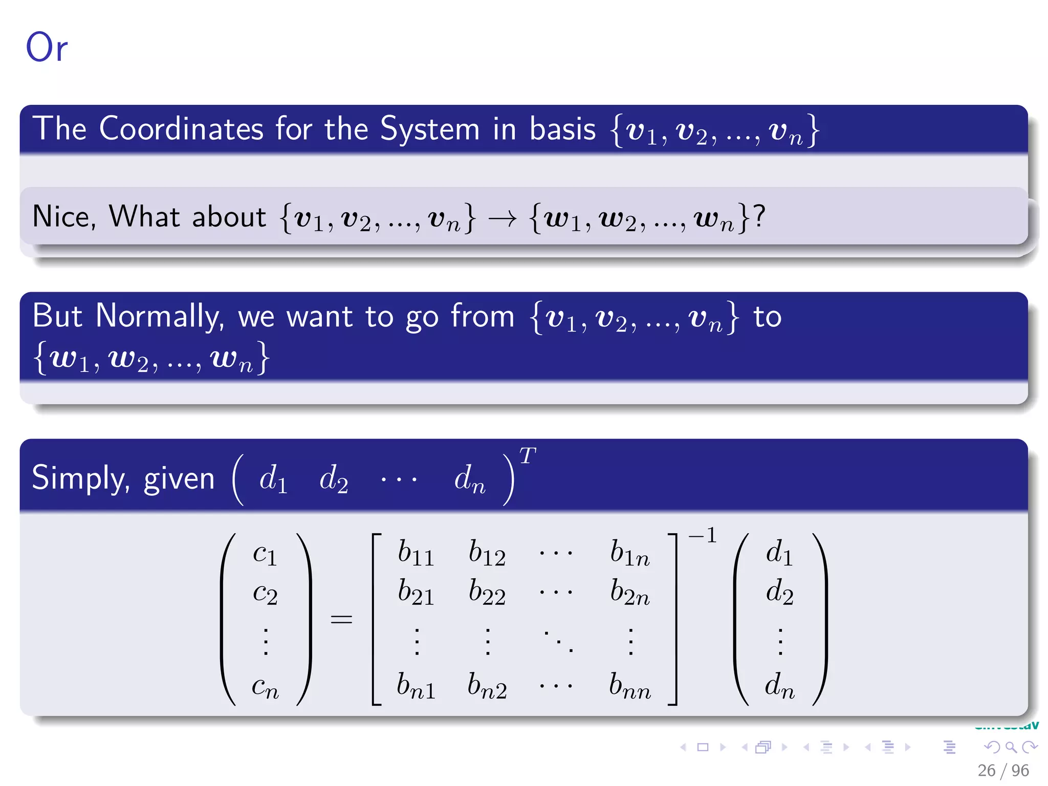
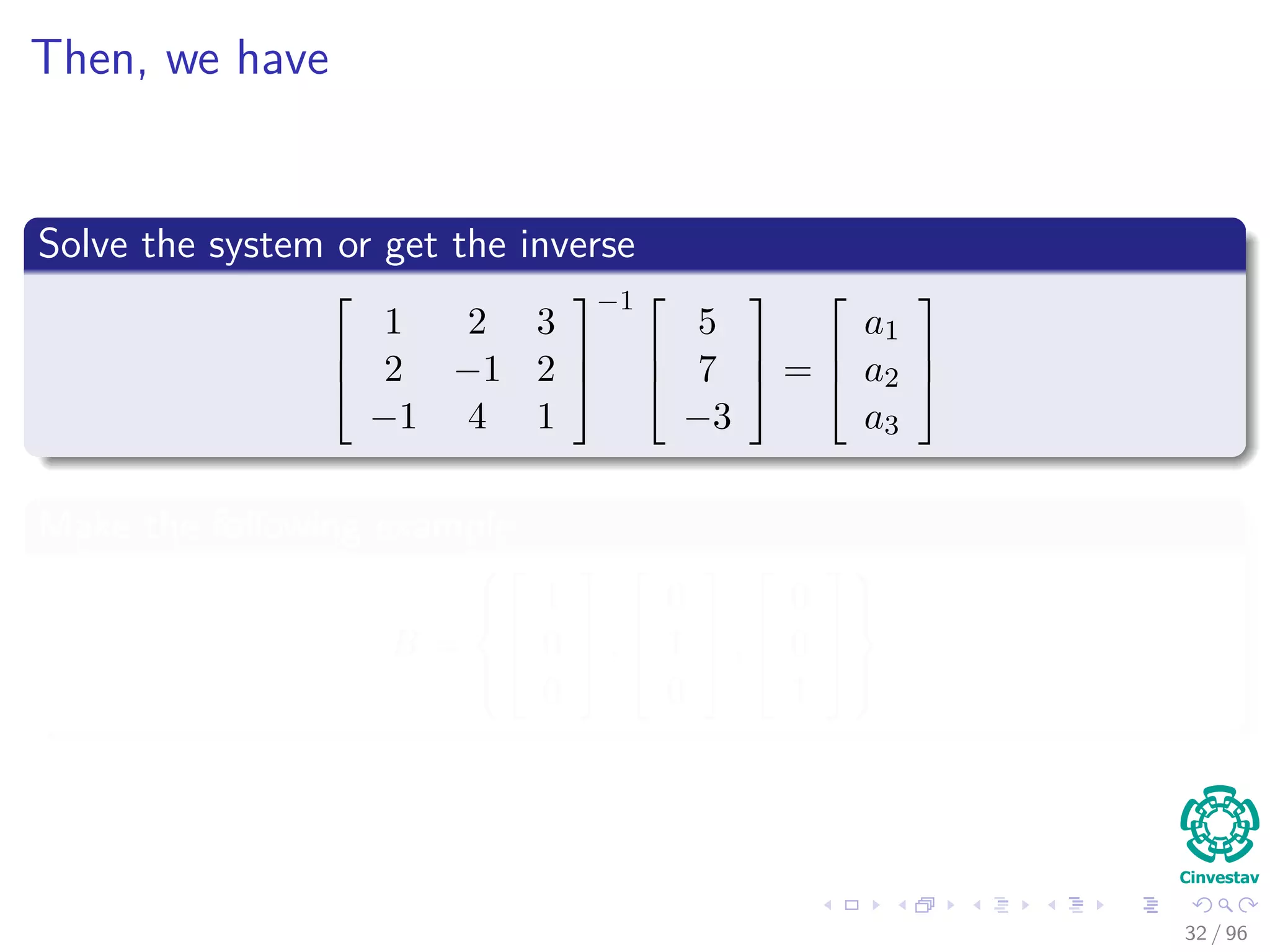
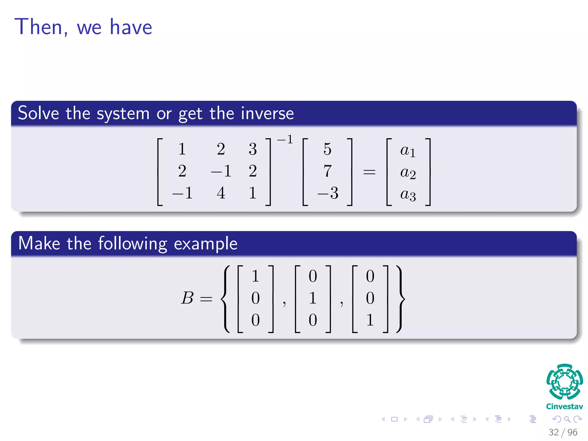
![Now, we have that to move from one basis to another
What if we have a element in basis S
[v]S =
5
7
−3
We derive the B coordinates of vector v
5
7
−3
==
1 2 3
2 −1 2
−1 4 1
a1
a2
a3
31 / 96](https://image.slidesharecdn.com/01-200420204420/75/01-02-linear-equations-49-2048.jpg)
![Now, we have that to move from one basis to another
What if we have a element in basis S
[v]S =
5
7
−3
We derive the B coordinates of vector v
5
7
−3
==
1 2 3
2 −1 2
−1 4 1
a1
a2
a3
31 / 96](https://image.slidesharecdn.com/01-200420204420/75/01-02-linear-equations-50-2048.jpg)
![Change of basis from B to B
Given an old basis B of Rn
with transition matrix PB
And a new basis B with transition matrix PB
How do we change from coords in the basis B to coords in the basis
B ?
Coordinates in B, then using v = PB [v]B we change the coordinates
to standard coordinates.
Then, we can do
[v]B = P−1
B v
33 / 96](https://image.slidesharecdn.com/01-200420204420/75/01-02-linear-equations-53-2048.jpg)
![Change of basis from B to B
Given an old basis B of Rn
with transition matrix PB
And a new basis B with transition matrix PB
How do we change from coords in the basis B to coords in the basis
B ?
Coordinates in B, then using v = PB [v]B we change the coordinates
to standard coordinates.
Then, we can do
[v]B = P−1
B v
33 / 96](https://image.slidesharecdn.com/01-200420204420/75/01-02-linear-equations-54-2048.jpg)
![Change of basis from B to B
Given an old basis B of Rn
with transition matrix PB
And a new basis B with transition matrix PB
How do we change from coords in the basis B to coords in the basis
B ?
Coordinates in B, then using v = PB [v]B we change the coordinates
to standard coordinates.
Then, we can do
[v]B = P−1
B v
33 / 96](https://image.slidesharecdn.com/01-200420204420/75/01-02-linear-equations-55-2048.jpg)
![Therefore, we have
We have the following situation
[v]B = P−1
B PB [v]B
Then, the final transition matrix
M = P−1
B PB = P−1
B v1 v2 · · · vn
In other words
M = P−1
B P−1
B v1 P−1
B v2 · · · P−1
B vn
34 / 96](https://image.slidesharecdn.com/01-200420204420/75/01-02-linear-equations-56-2048.jpg)
![Therefore, we have
We have the following situation
[v]B = P−1
B PB [v]B
Then, the final transition matrix
M = P−1
B PB = P−1
B v1 v2 · · · vn
In other words
M = P−1
B P−1
B v1 P−1
B v2 · · · P−1
B vn
34 / 96](https://image.slidesharecdn.com/01-200420204420/75/01-02-linear-equations-57-2048.jpg)
![Therefore, we have
We have the following situation
[v]B = P−1
B PB [v]B
Then, the final transition matrix
M = P−1
B PB = P−1
B v1 v2 · · · vn
In other words
M = P−1
B P−1
B v1 P−1
B v2 · · · P−1
B vn
34 / 96](https://image.slidesharecdn.com/01-200420204420/75/01-02-linear-equations-58-2048.jpg)
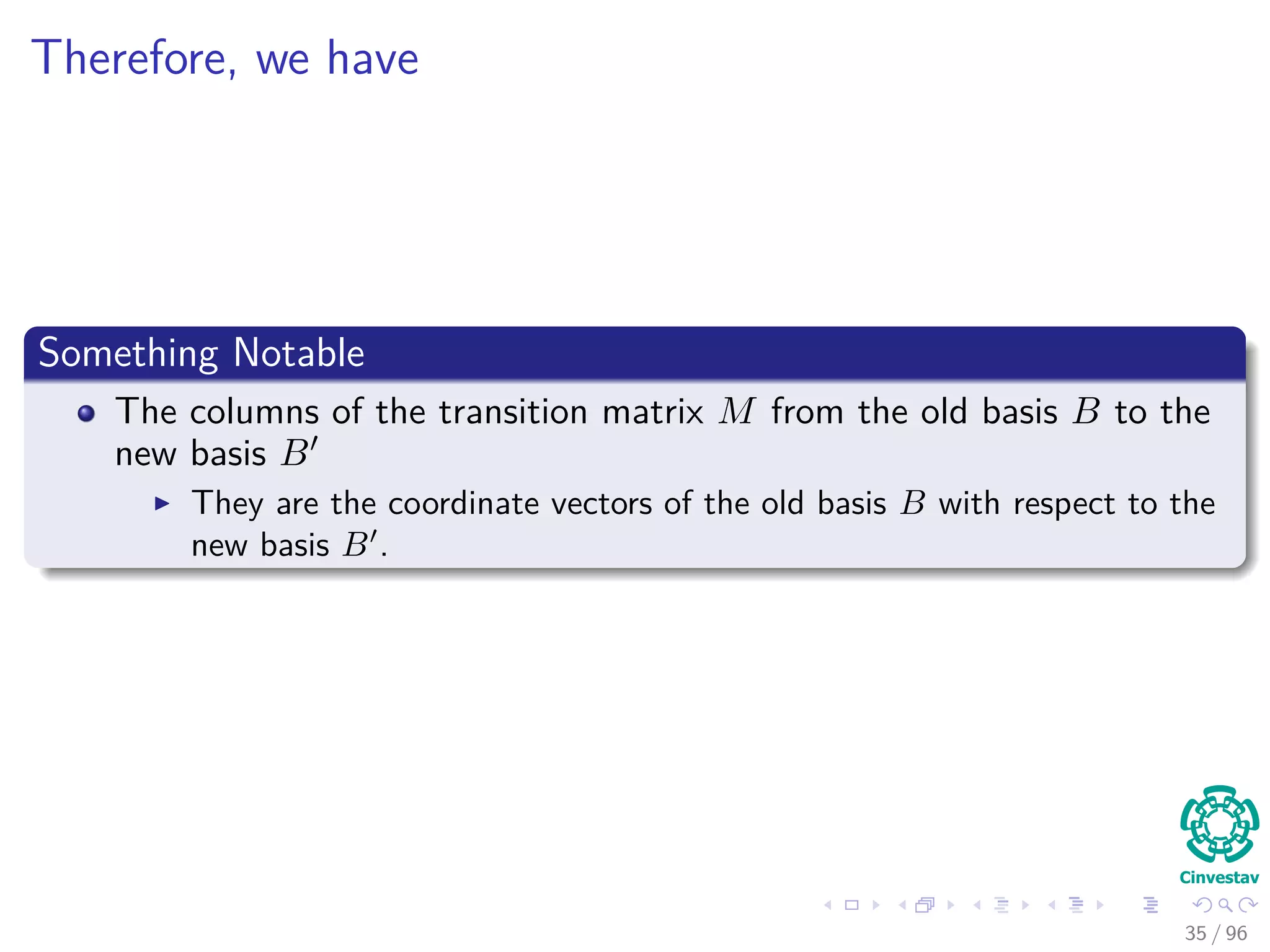
![Fianlly, packing everything
Theorem
If B and B are two bases of Rn , with B = {v1, v2, · · · , vn} then
the transition matrix from B coordinates to B coordinates is given by
M = [[v1]B , [v2]B , ..., [vn]B ]
36 / 96](https://image.slidesharecdn.com/01-200420204420/75/01-02-linear-equations-60-2048.jpg)
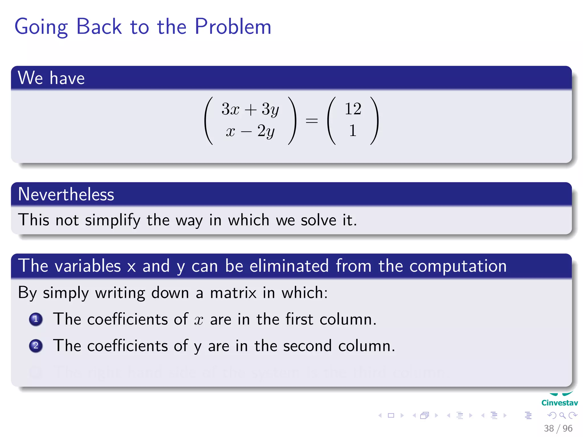
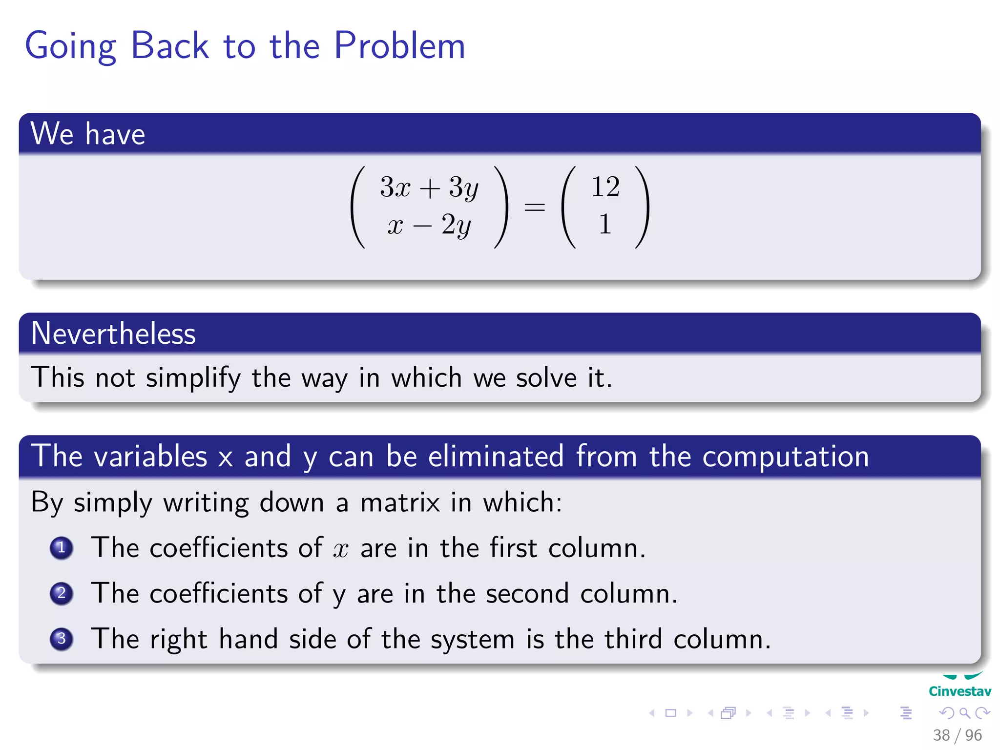
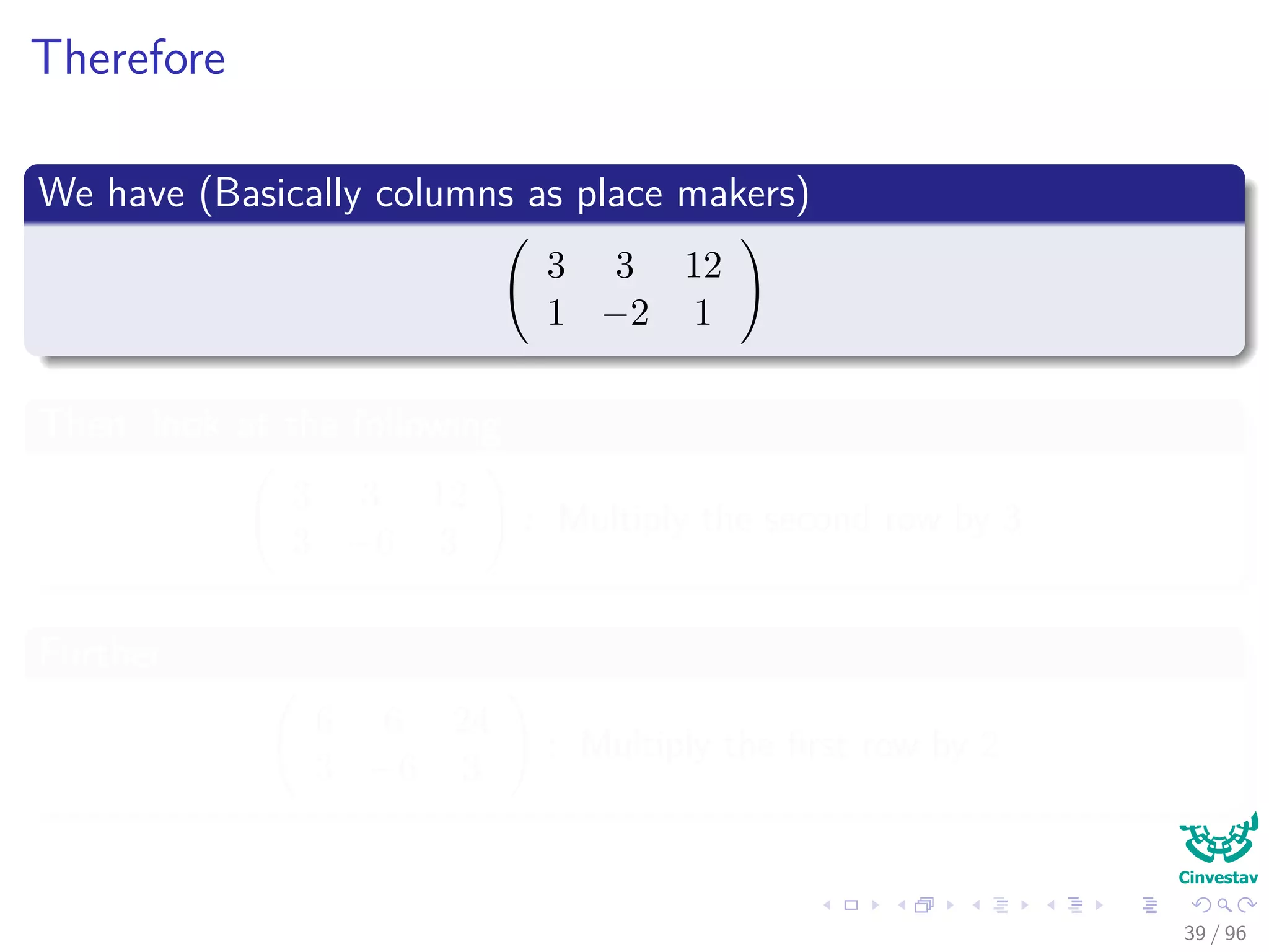
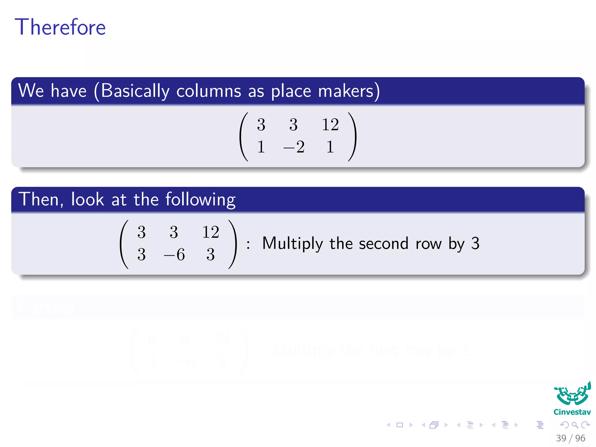
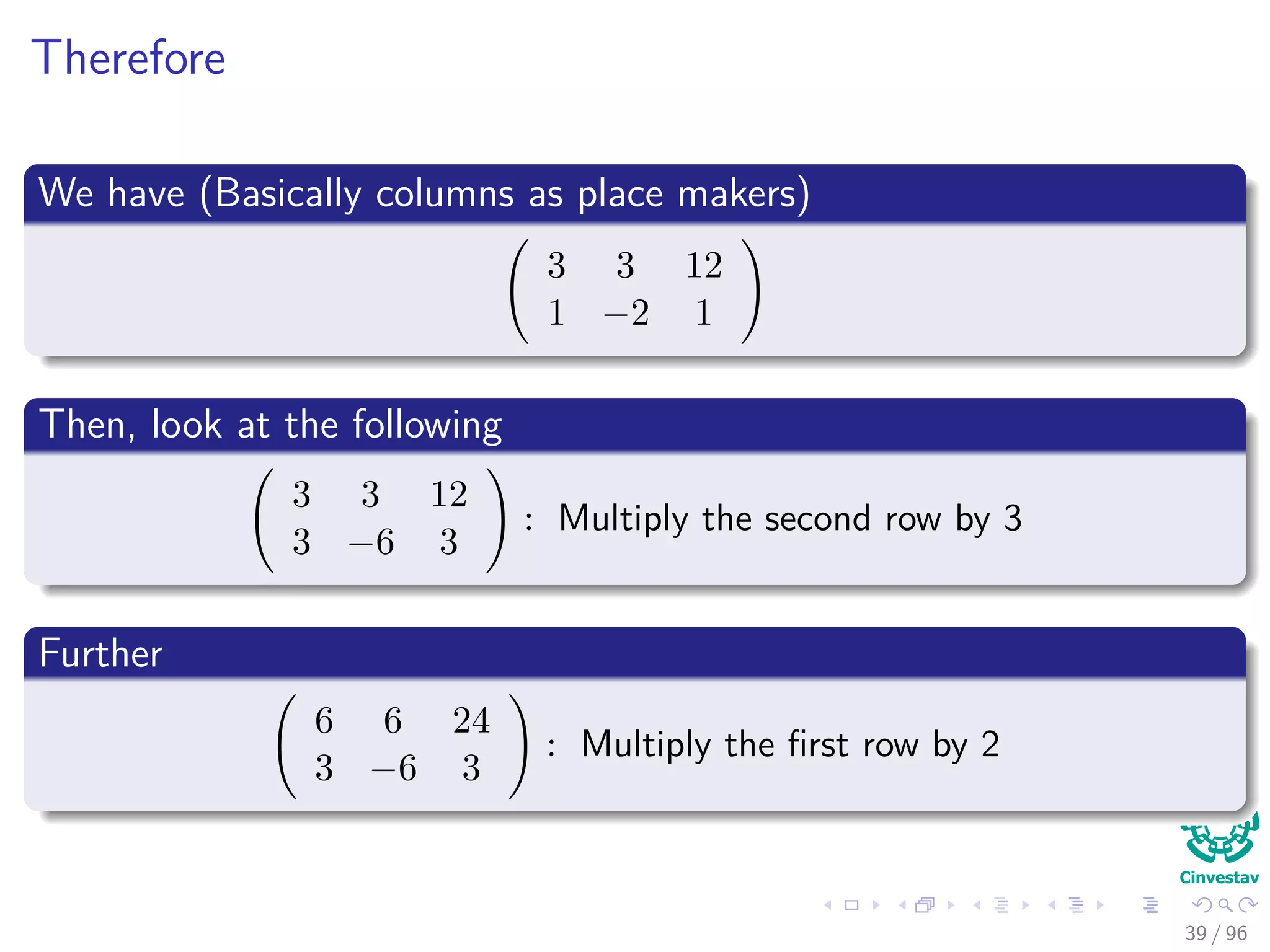

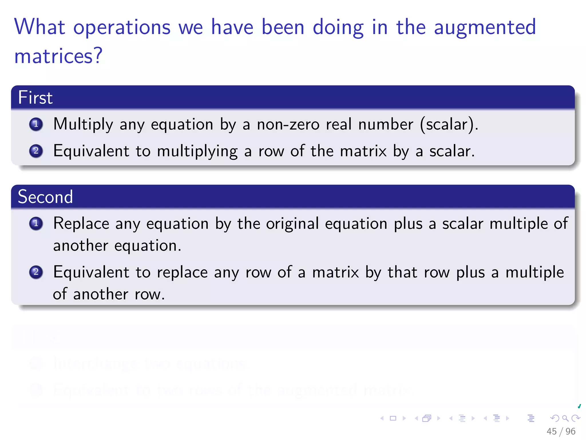
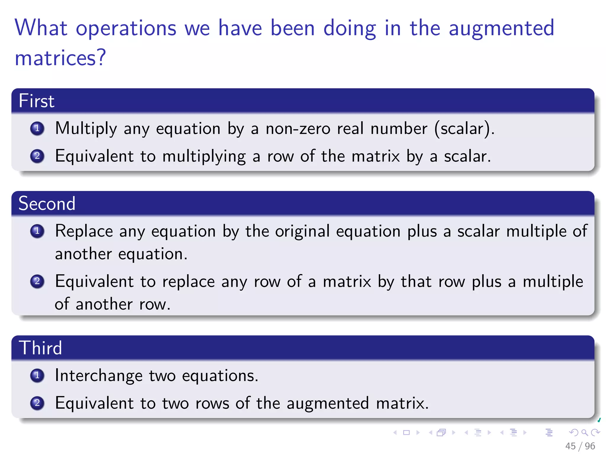
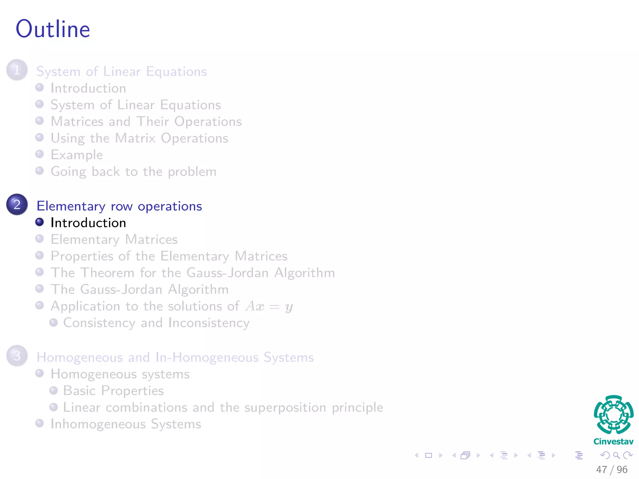


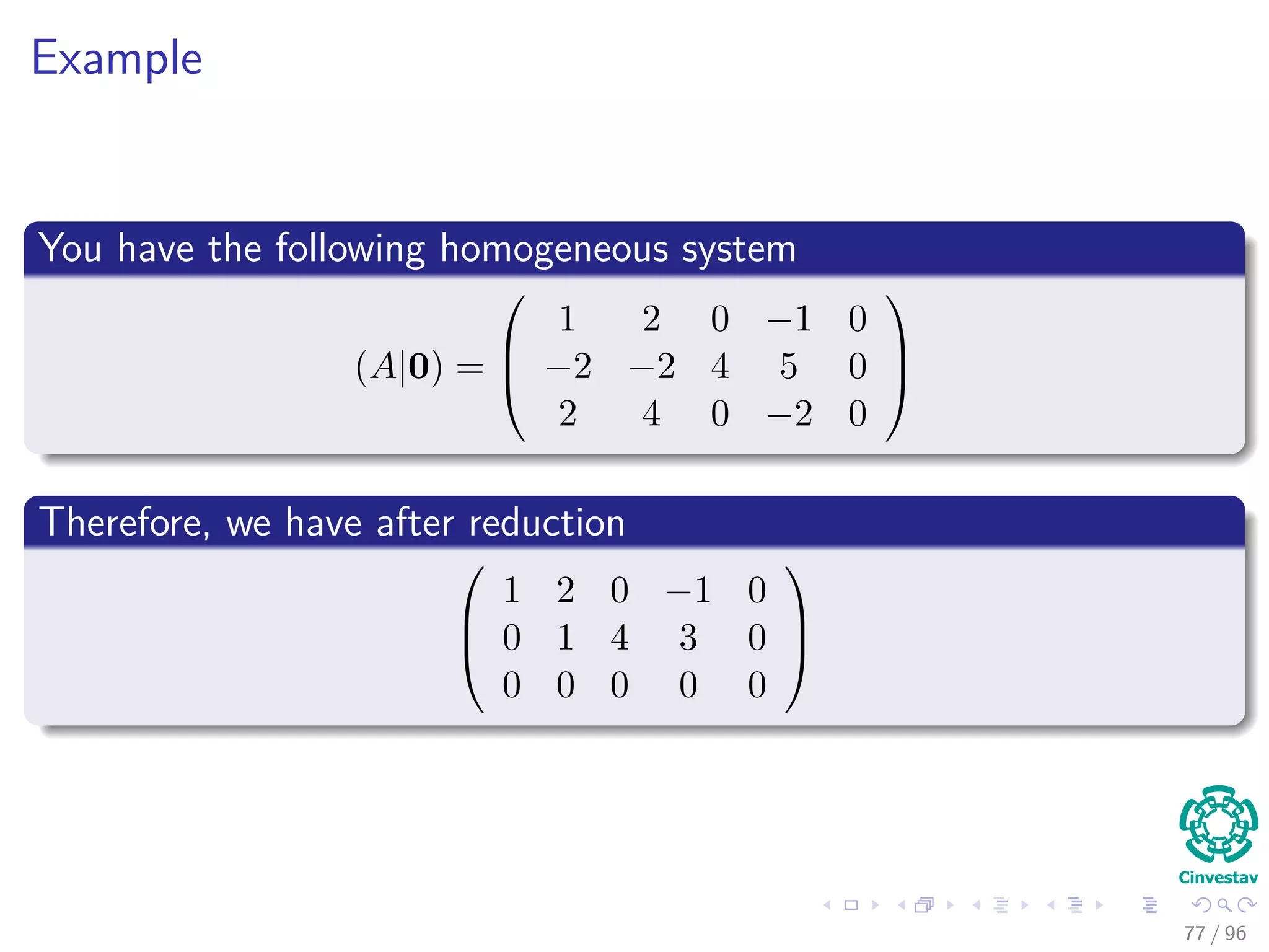
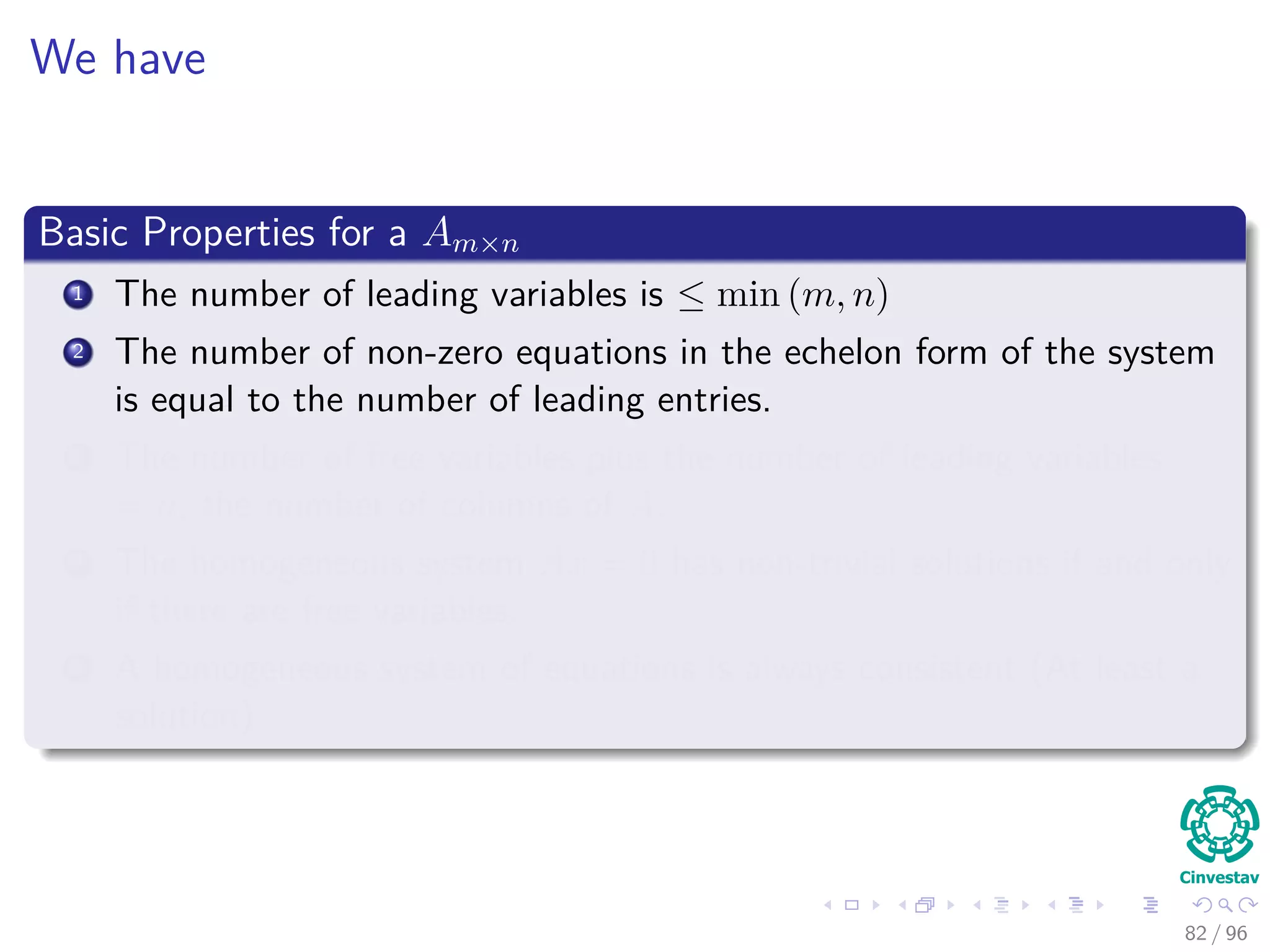
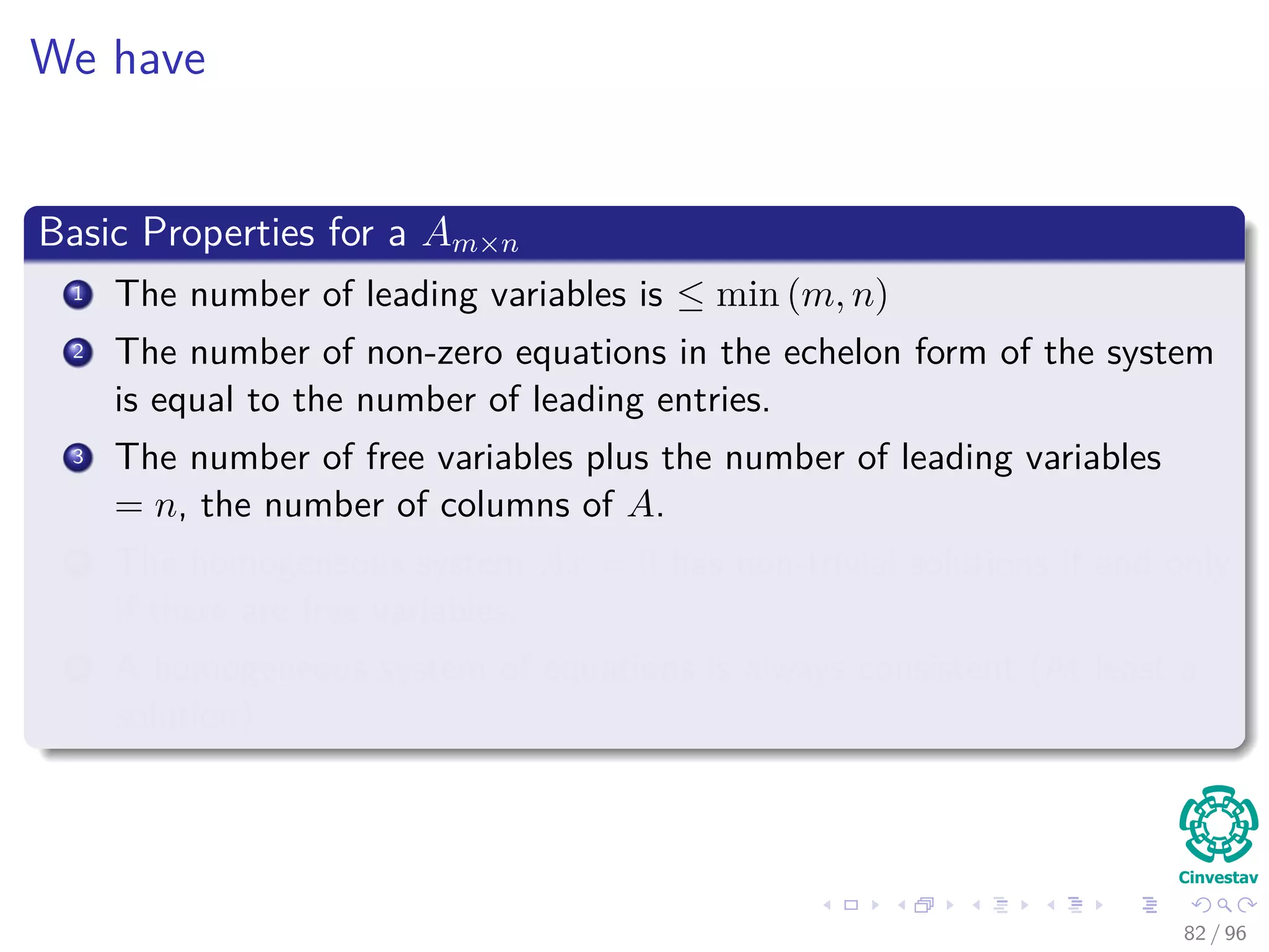
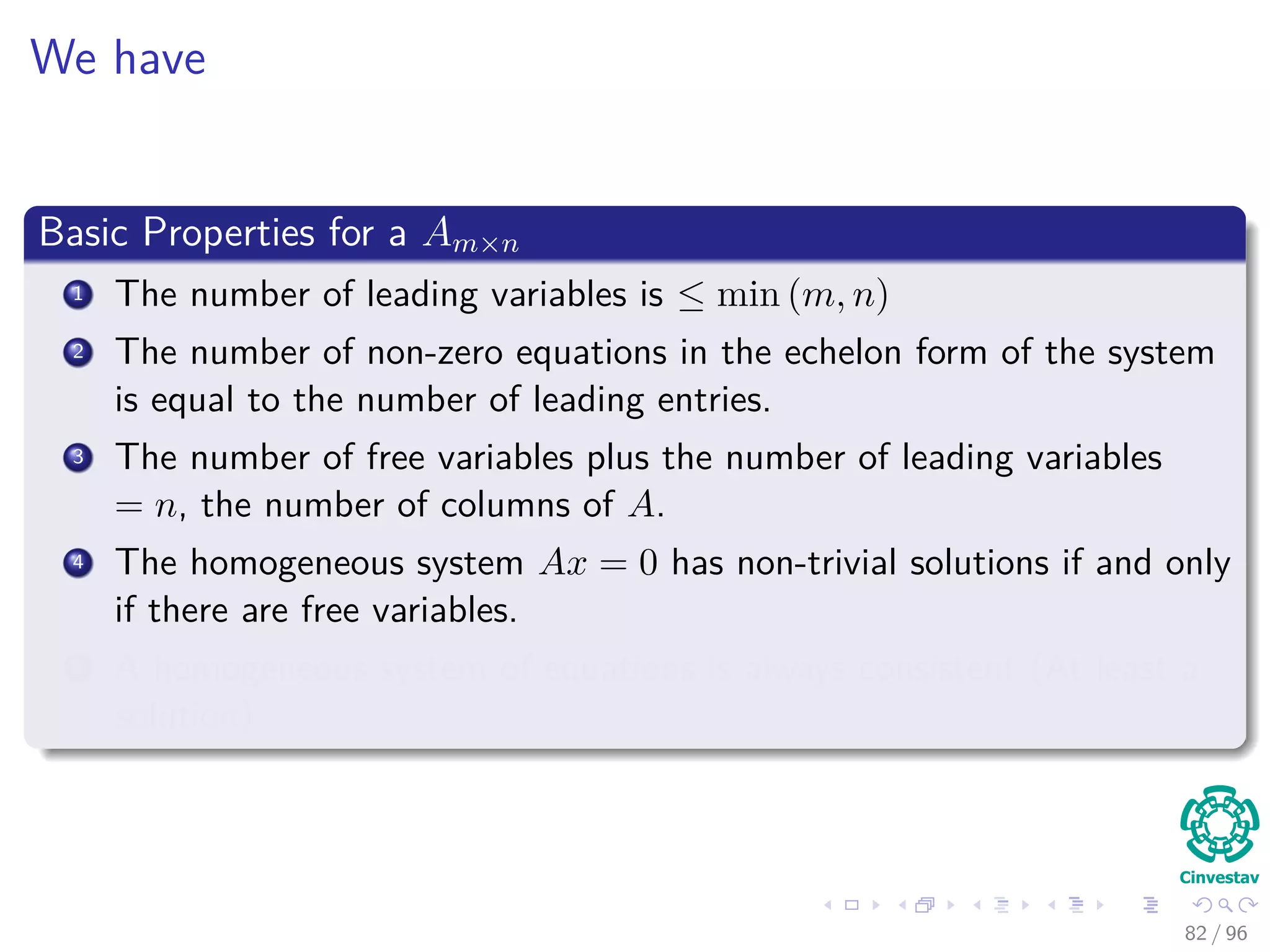
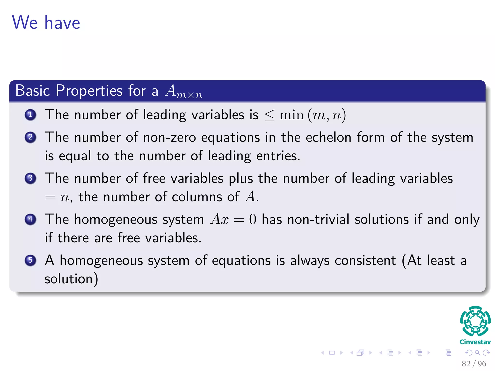

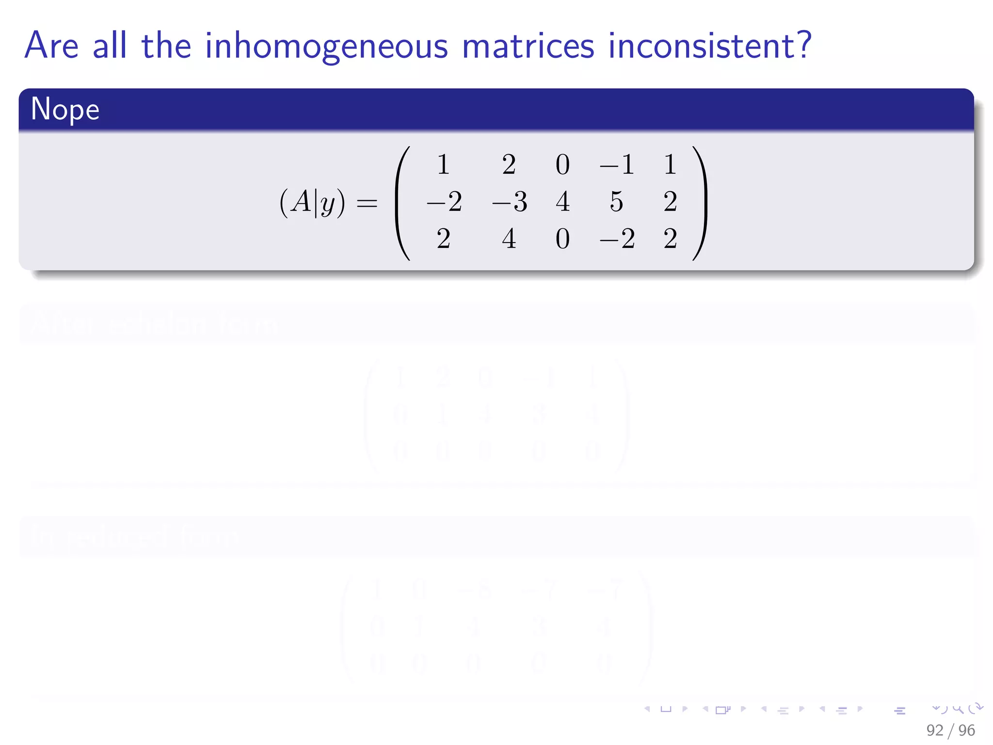
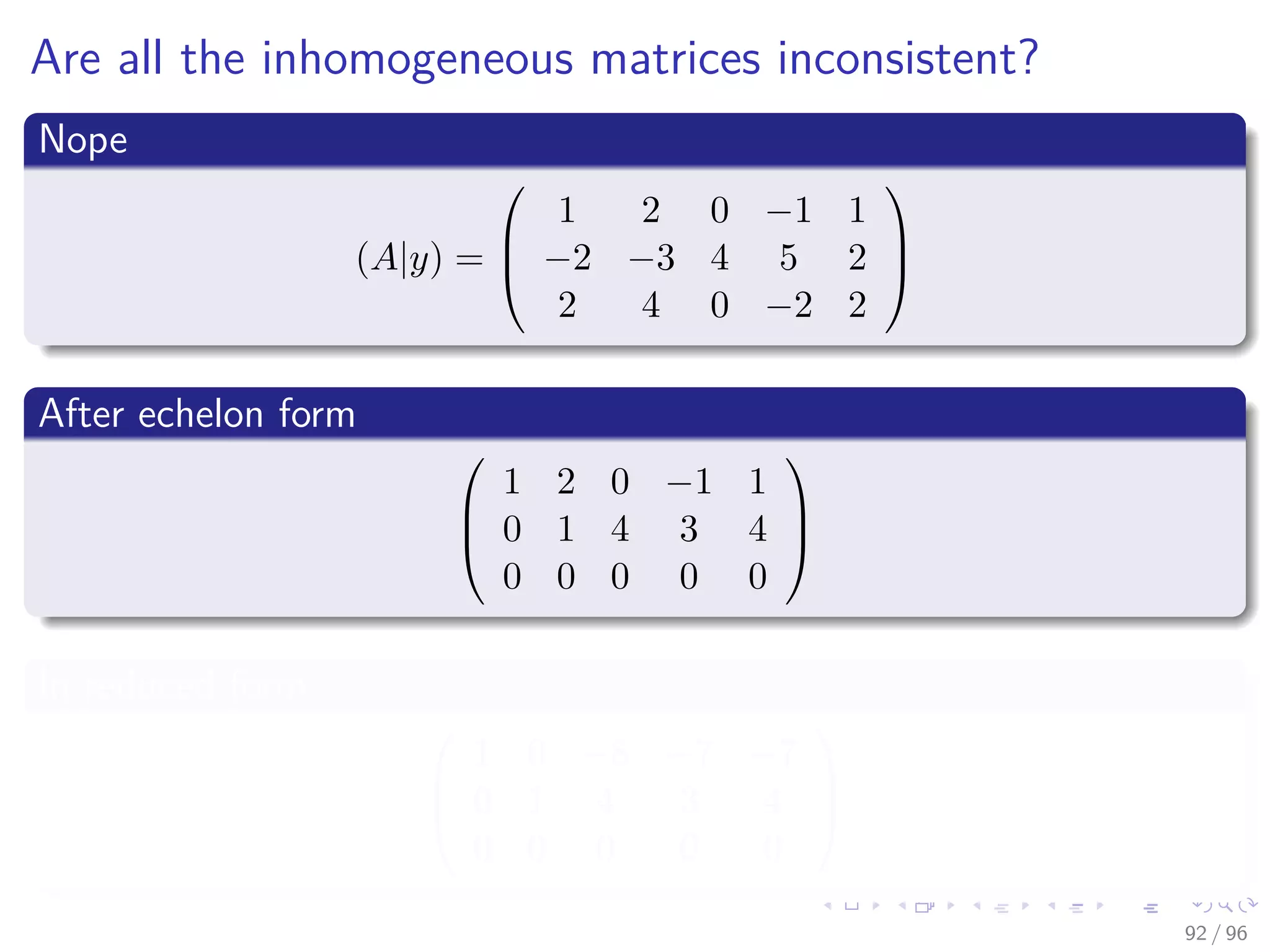
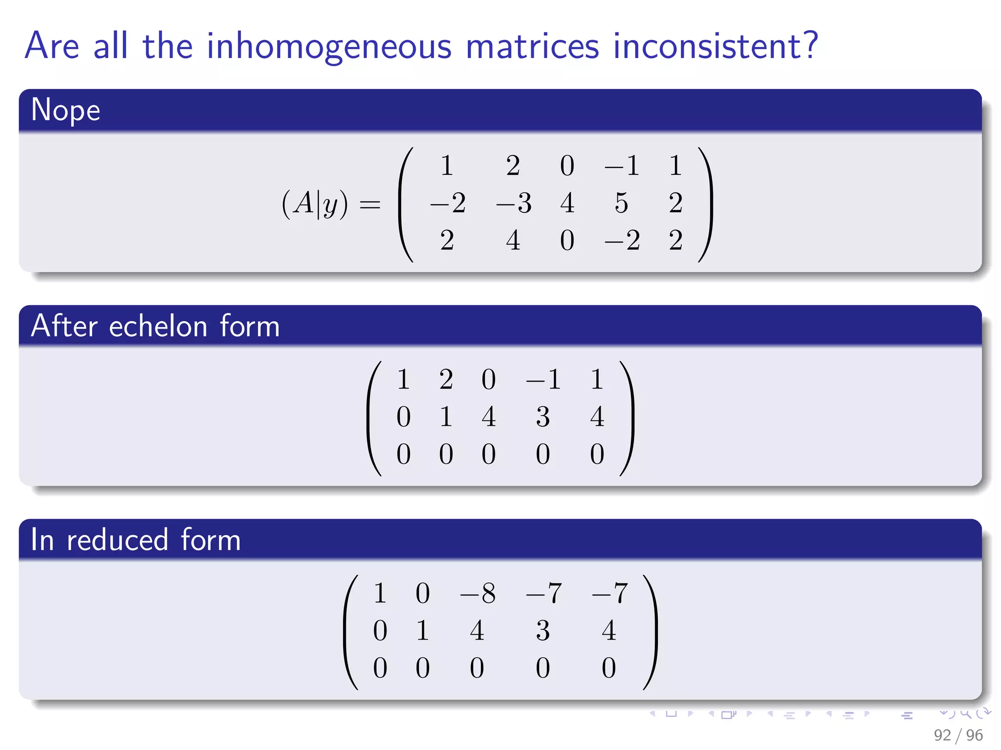


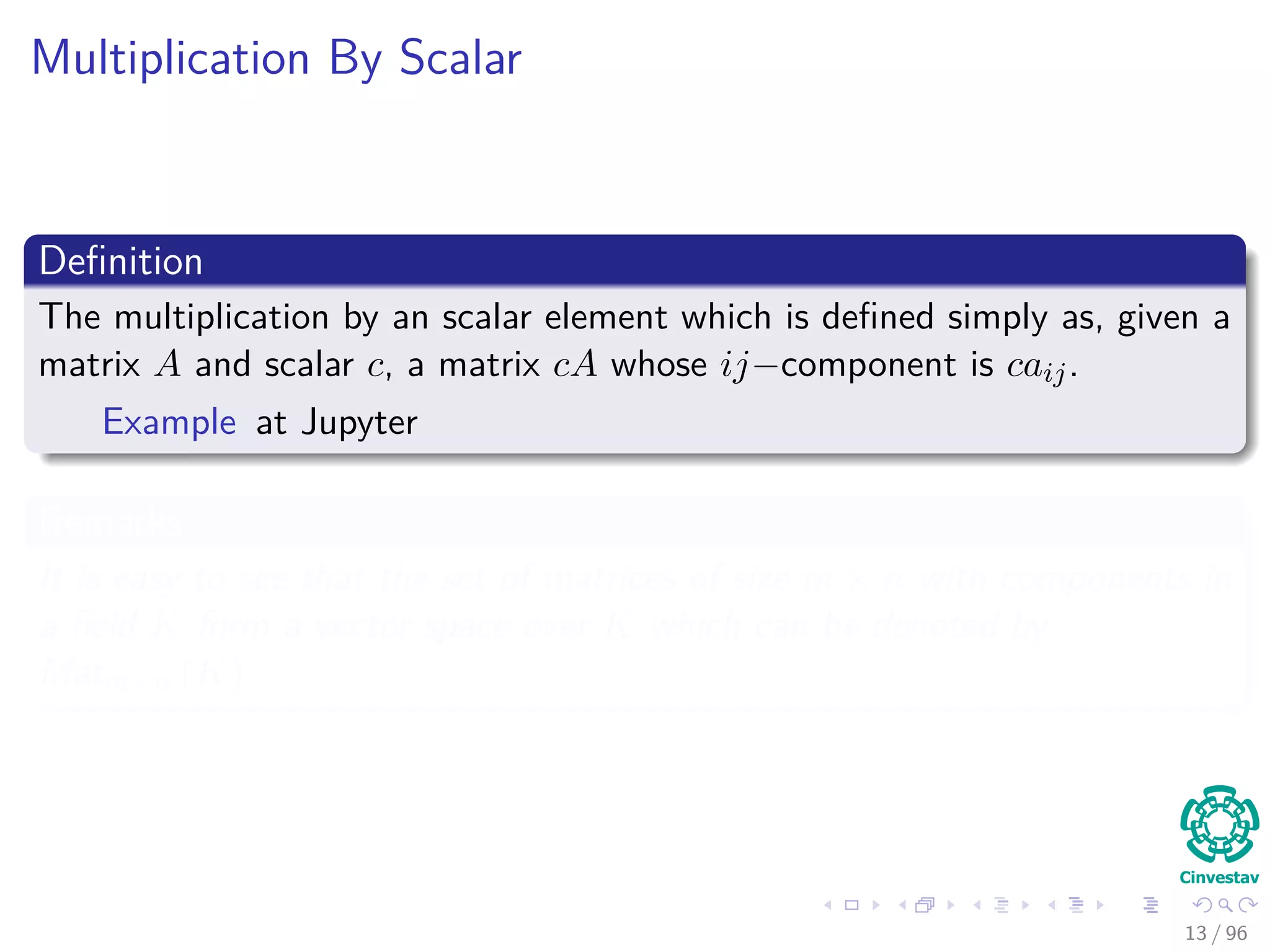
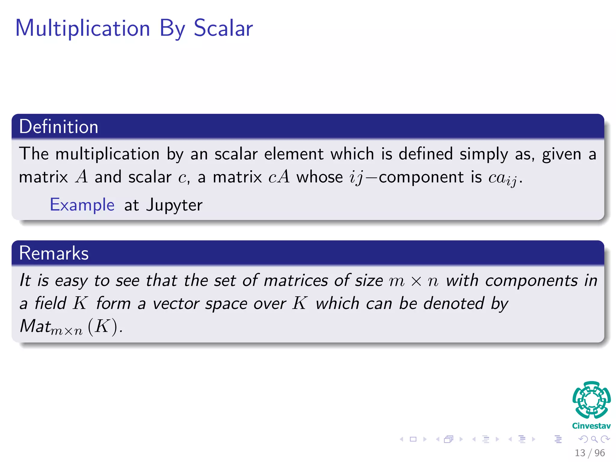
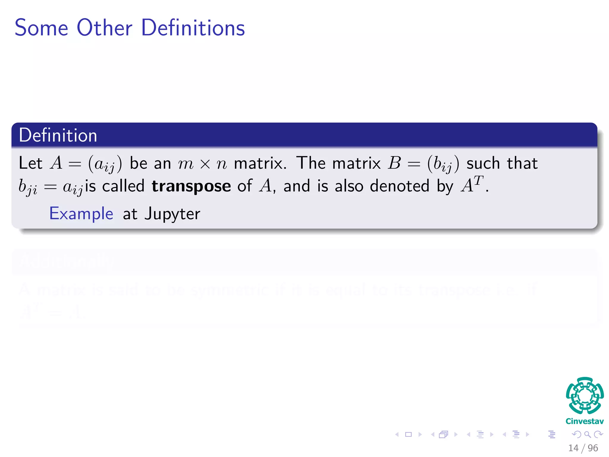
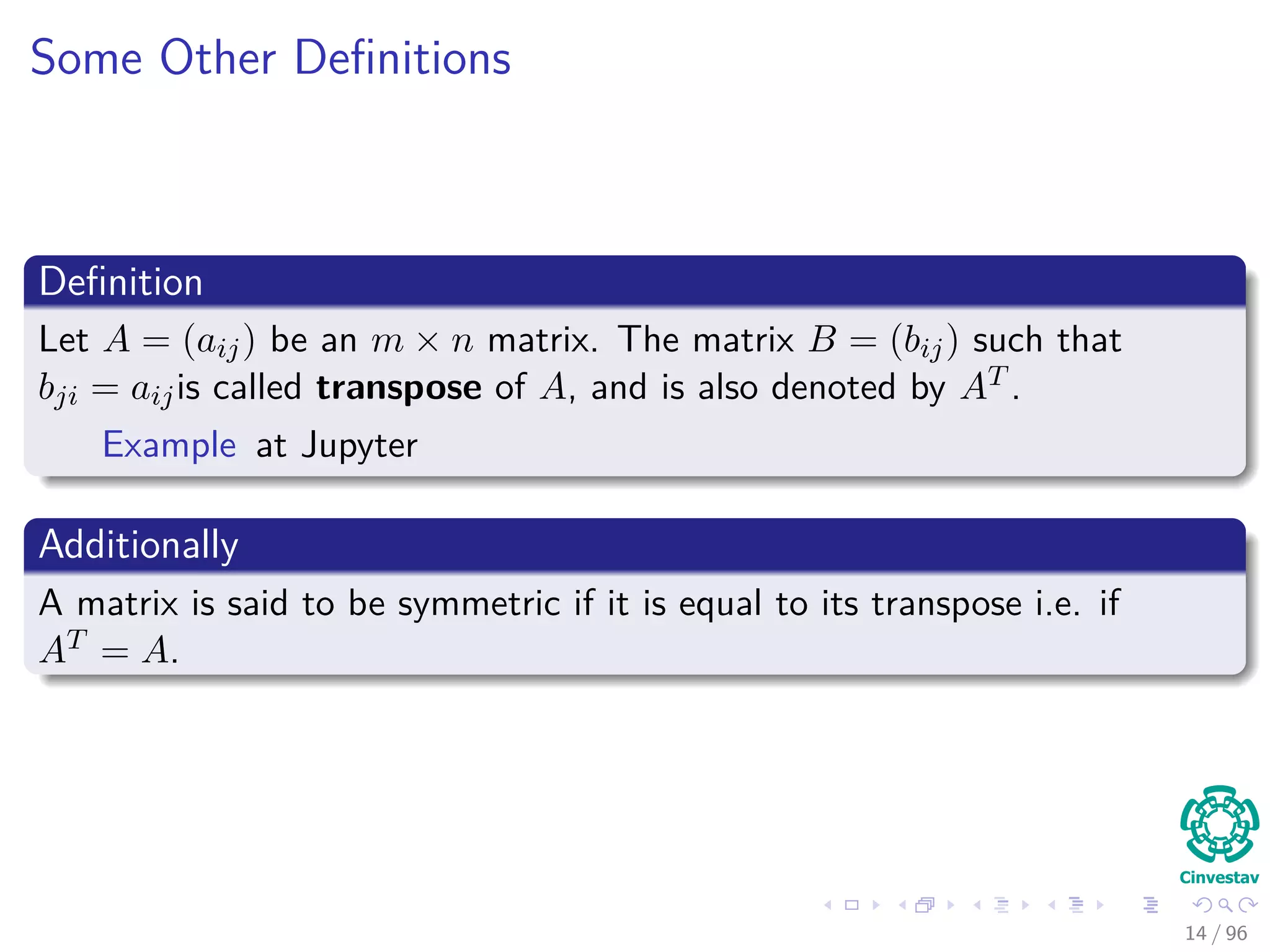
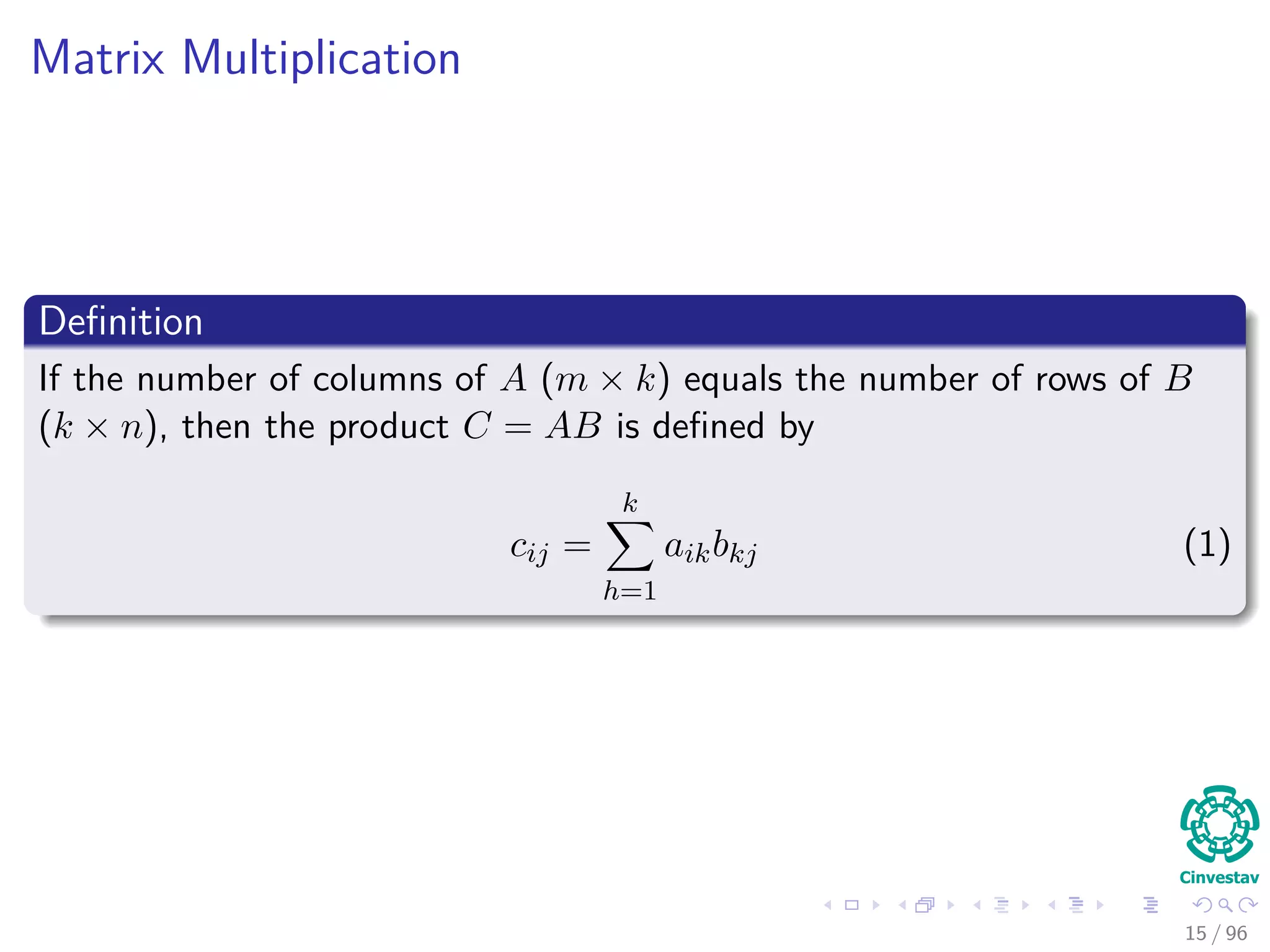
This document provides an introduction to systems of linear equations and matrix operations. It defines key concepts such as matrices, matrix addition and multiplication, and transitions between different bases. It presents an example of multiplying two matrices using NumPy. The document outlines how systems of linear equations can be represented using matrices and discusses solving systems using techniques like Gauss-Jordan elimination and elementary row operations. It also introduces the concepts of homogeneous and inhomogeneous systems.