Matrices
•Basics
•Types
•Operations
•Multiplication
•Determinant
•Inverse
•Eigen Values
•Linear Equations
•RANK
Matrices - Introduction
Matrix algebra has at least two advantages:
•Reduces complicated systems of equations to simple
expressions
•Adaptable to systematic method of mathematical treatment
and well suited to computers
Definition:
A matrix is a set or group of numbers arranged in a square or
rectangular array enclosed by two brackets
 
1
1  





 0
3
2
4






d
c
b
a
Matrices - Introduction
Properties:
•A specified number of rows and a specified number of
columns
•Two numbers (rows x columns) describe the dimensions
or size of the matrix.
Examples:
3x3 matrix
2x4 matrix
1x2 matrix 










3
3
3
5
1
4
4
2
1





 
2
3
3
3
0
1
0
1
 
1
1 
Matrices - Introduction
TYPES OF MATRICES
1. Column matrix or vector:
The number of rows may be any integer but the number of
columns is always 1










2
4
1






3
1












1
21
11
m
a
a
a

Matrices - Introduction
TYPES OF MATRICES
2. Row matrix or vector
Any number of columns but only one row
 
6
1
1  
2
5
3
0
 
n
a
a
a
a 1
13
12
11 
Matrices - Introduction
TYPES OF MATRICES
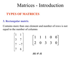
3. Rectangular matrix
Contains more than one element and number of rows is not
equal to the number of columns













6
7
7
7
7
3
1
1






0
3
3
0
2
0
0
1
1
1
n
m
Matrices - Introduction
TYPES OF MATRICES
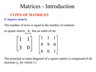
4. Square matrix
The number of rows is equal to the number of columns
(a square matrix A has an order of m)






0
3
1
1










1
6
6
0
9
9
1
1
1
m x m
The principal or main diagonal of a square matrix is composed of all
elements aij for which i=j
Matrices - Introduction
TYPES OF MATRICES
5. Diagonal matrix
A square matrix where all the elements are zero except those on
the main diagonal










1
0
0
0
2
0
0
0
1












9
0
0
0
0
5
0
0
0
0
3
0
0
0
0
3
i.e. aij =0 for all i = j
aij = 0 for some or all i = j
Matrices - Introduction
TYPES OF MATRICES
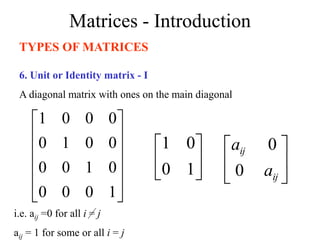
6. Unit or Identity matrix - I
A diagonal matrix with ones on the main diagonal












1
0
0
0
0
1
0
0
0
0
1
0
0
0
0
1






1
0
0
1
i.e. aij =0 for all i = j
aij = 1 for some or all i = j






ij
ij
a
a
0
0
Matrices - Introduction
TYPES OF MATRICES
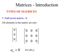
7. Null (zero) matrix - 0
All elements in the matrix are zero










0
0
0










0
0
0
0
0
0
0
0
0
0

ij
a For all i,j
Matrices - Introduction
TYPES OF MATRICES
8. Triangular matrix
A square matrix whose elements above or below the main
diagonal are all zero










3
2
5
0
1
2
0
0
1










3
2
5
0
1
2
0
0
1










3
0
0
6
1
0
9
8
1
Matrices - Introduction
TYPES OF MATRICES
8a. Upper triangular matrix
A square matrix whose elements below the main
diagonal are all zero
i.e. aij = 0 for all i > j










3
0
0
8
1
0
7
8
1












3
0
0
0
8
7
0
0
4
7
1
0
4
4
7
1










ij
ij
ij
ij
ij
ij
a
a
a
a
a
a
0
0
0
Matrices - Introduction
TYPES OF MATRICES
A square matrix whose elements above the main diagonal are all
zero
8b. Lower triangular matrix
i.e. aij = 0 for all i < j










3
2
5
0
1
2
0
0
1










ij
ij
ij
ij
ij
ij
a
a
a
a
a
a
0
0
0
Matrices – Introduction
TYPES OF MATRICES
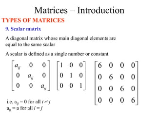
9. Scalar matrix
A diagonal matrix whose main diagonal elements are
equal to the same scalar
A scalar is defined as a single number or constant










1
0
0
0
1
0
0
0
1












6
0
0
0
0
6
0
0
0
0
6
0
0
0
0
6
i.e. aij = 0 for all i = j
aij = a for all i = j










ij
ij
ij
a
a
a
0
0
0
0
0
0
Matrices - Operations
EQUALITY OF MATRICES
Two matrices are said to be equal only when all
corresponding elements are equal
Therefore their size or dimensions are equal as well










3
2
5
0
1
2
0
0
1










3
2
5
0
1
2
0
0
1
A = B = A = B
Matrices - Operations
Some properties of equality:
•IIf A = B, then B = A for all A and B
•IIf A = B, and B = C, then A = C for all A, B and C










3
2
5
0
1
2
0
0
1
A = B =










33
32
31
23
22
21
13
12
11
b
b
b
b
b
b
b
b
b
If A = B then ij
ij b
a 
Matrices - Operations
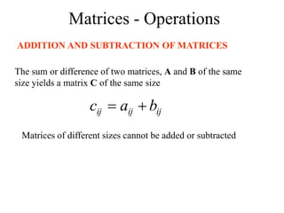
ADDITION AND SUBTRACTION OF MATRICES
The sum or difference of two matrices, A and B of the same
size yields a matrix C of the same size
ij
ij
ij b
a
c 

Matrices of different sizes cannot be added or subtracted
Matrices - Operations
SCALAR MULTIPLICATION OF MATRICES
Matrices can be multiplied by a scalar (constant or single
element)
Let k be a scalar quantity; then
kA = Ak
Ex. If k=4 and















1
4
3
2
1
2
1
3
A
Matrices - Operations














































4
16
12
8
4
8
4
12
4
1
4
3
2
1
2
1
3
1
4
3
2
1
2
1
3
4
Properties:
• k (A + B) = kA + kB
• (k + g)A = kA + gA
• k(AB) = (kA)B = A(k)B
• k(gA) = (kg)A
Matrices - Operations
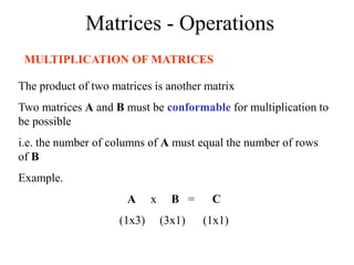
MULTIPLICATION OF MATRICES
The product of two matrices is another matrix
Two matrices A and B must be conformable for multiplication to
be possible
i.e. the number of columns of A must equal the number of rows
of B
Example.
A x B = C
(1x3) (3x1) (1x1)
Matrices - Operations
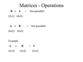
B x A = Not possible!
(2x1) (4x2)
A x B = Not possible!
(6x2) (6x3)
Example
A x B = C
(2x3) (3x2) (2x2)
Matrices - Operations























22
21
12
11
32
31
22
21
12
11
23
22
21
13
12
11
c
c
c
c
b
b
b
b
b
b
a
a
a
a
a
a
22
32
23
22
22
12
21
21
31
23
21
22
11
21
12
32
13
22
12
12
11
11
31
13
21
12
11
11
)
(
)
(
)
(
)
(
)
(
)
(
)
(
)
(
)
(
)
(
)
(
)
(
c
b
a
b
a
b
a
c
b
a
b
a
b
a
c
b
a
b
a
b
a
c
b
a
b
a
b
a
























Successive multiplication of row i of A with column j of
B – row by column multiplication
Matrices - Operations











































)
3
7
(
)
2
2
(
)
8
4
(
)
5
7
(
)
6
2
(
)
4
4
(
)
3
3
(
)
2
2
(
)
8
1
(
)
5
3
(
)
6
2
(
)
4
1
(
3
5
2
6
8
4
7
2
4
3
2
1







57
63
21
31
Remember also:
IA = A






1
0
0
1






57
63
21
31







57
63
21
31
Matrices - Operations
Assuming that matrices A, B and C are conformable for
the operations indicated, the following are true:
1. AI = IA = A
2. A(BC) = (AB)C = ABC - (associative law)
3. A(B+C) = AB + AC - (first distributive law)
4. (A+B)C = AC + BC - (second distributive law)
Caution!
1. AB not generally equal to BA, BA may not be conformable
2. If AB = 0, neither A nor B necessarily = 0
3. If AB = AC, B not necessarily = C
Matrices - Operations
If AB = 0, neither A nor B necessarily = 0





















0
0
0
0
3
2
3
2
0
0
1
1
Matrices - Operations
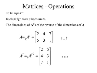
To transpose:
Interchange rows and columns
The dimensions of AT are the reverse of the dimensions of A








1
3
5
7
4
2
3
2A
A












1
7
3
4
5
2
2
3
T
T
A
A
2 x 3
3 x 2
Matrices - Operations
Properties of transposed matrices:
1. (A+B)T = AT + BT
2. (AB)T = BT AT
3. (kA)T = kAT
4. (AT)T = A
Matrices - Operations
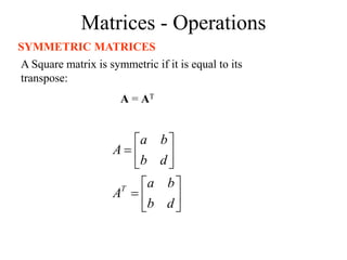
SYMMETRIC MATRICES
A Square matrix is symmetric if it is equal to its
transpose:
A = AT














d
b
b
a
A
d
b
b
a
A
T
Matrices - Operations
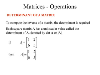
DETERMINANT OF A MATRIX
To compute the inverse of a matrix, the determinant is required
Each square matrix A has a unit scalar value called the
determinant of A, denoted by det A or |A|
5
6
2
1
5
6
2
1








A
A
If
then
Matrices - Operations
If A = [A] is a single element (1x1), then the determinant is
defined as the value of the element
Then |A| =det A = a11
If A is (n x n), its determinant may be defined in terms of order
(n-1) or less.
Matrices - Operations
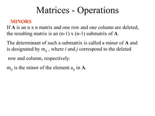
MINORS
If A is an n x n matrix and one row and one column are deleted,
the resulting matrix is an (n-1) x (n-1) submatrix of A.
The determinant of such a submatrix is called a minor of A and
is designated by mij , where i and j correspond to the deleted
row and column, respectively.
mij is the minor of the element aij in A.
Matrices - Operations











33
32
31
23
22
21
13
12
11
a
a
a
a
a
a
a
a
a
A
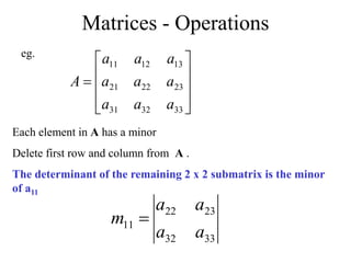
Each element in A has a minor
Delete first row and column from A .
The determinant of the remaining 2 x 2 submatrix is the minor
of a11
eg.
33
32
23
22
11
a
a
a
a
m 
Matrices - Operations
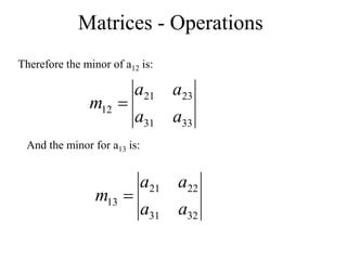
Therefore the minor of a12 is:
And the minor for a13 is:
33
31
23
21
12
a
a
a
a
m 
32
31
22
21
13
a
a
a
a
m 
Matrices - Operations
COFACTORS
The cofactor Cij of an element aij is defined as:
ij
j
i
ij m
C 

 )
1
(
When the sum of a row number i and column j is even, cij = mij and
when i+j is odd, cij =-mij
13
13
3
1
13
12
12
2
1
12
11
11
1
1
11
)
1
(
)
3
,
1
(
)
1
(
)
2
,
1
(
)
1
(
)
1
,
1
(
m
m
j
i
c
m
m
j
i
c
m
m
j
i
c





















Matrices - Operations
DETERMINANTS CONTINUED
The determinant of an n x n matrix A can now be defined as
n
nc
a
c
a
c
a
A
A 1
1
12
12
11
11
det 



 
The determinant of A is therefore the sum of the products of the
elements of the first row of A and their corresponding cofactors.
(It is possible to define |A| in terms of any other row or column
but for simplicity, the first row only is used)
Matrices - Operations
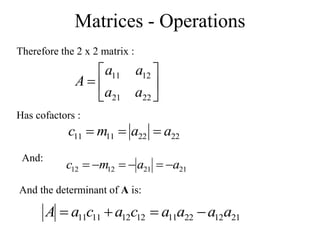
Therefore the 2 x 2 matrix :







22
21
12
11
a
a
a
a
A
Has cofactors :
22
22
11
11 a
a
m
c 


And:
21
21
12
12 a
a
m
c 





And the determinant of A is:
21
12
22
11
12
12
11
11 a
a
a
a
c
a
c
a
A 



Matrices - Operations
Example 1:







2
1
1
3
A
5
)
1
)(
1
(
)
2
)(
3
( 


A
Matrices - Operations
For a 3 x 3 matrix:











33
32
31
23
22
21
13
12
11
a
a
a
a
a
a
a
a
a
A
The cofactors of the first row are:
31
22
32
21
32
31
22
21
13
31
23
33
21
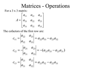
33
31
23
21
12
32
23
33
22
33
32
23
22
11
)
(
a
a
a
a
a
a
a
a
c
a
a
a
a
a
a
a
a
c
a
a
a
a
a
a
a
a
c











Matrices - Operations
The determinant of a matrix A is:
21
12
22
11
12
12
11
11 a
a
a
a
c
a
c
a
A 



Which by substituting for the cofactors in this case is:
)
(
)
(
)
( 31
22
32
21
13
31
23
33
21
12
32
23
33
22
11 a
a
a
a
a
a
a
a
a
a
a
a
a
a
a
A 





Matrices - Operations
Example 2:












1
0
1
3
2
0
1
0
1
A
4
)
2
0
)(
1
(
)
3
0
)(
0
(
)
0
2
)(
1
( 






A
)
(
)
(
)
( 31
22
32
21
13
31
23
33
21
12
32
23
33
22
11 a
a
a
a
a
a
a
a
a
a
a
a
a
a
a
A 





Matrices - Operations
ADJOINT MATRICES
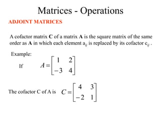
A cofactor matrix C of a matrix A is the square matrix of the same
order as A in which each element aij is replaced by its cofactor cij .
Example:








4
3
2
1
A








1
2
3
4
C
If
The cofactor C of A is
Matrices - Operations
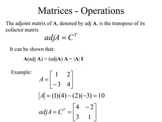
The adjoint matrix of A, denoted by adj A, is the transpose of its
cofactor matrix
T
C
adjA 
It can be shown that:
A(adj A) = (adjA) A = |A| I
Example:





 














1
3
2
4
10
)
3
)(
2
(
)
4
)(
1
(
4
3
2
1
T
C
adjA
A
A
Matrices - Operations
I
adjA
A 10
10
0
0
10
1
3
2
4
4
3
2
1
)
( 












 








I
A
adjA 10
10
0
0
10
4
3
2
1
1
3
2
4
)
( 



















 

Matrices - Operations
USING THE ADJOINT MATRIX IN MATRIX INVERSION
A
adjA
A 
1
Since
AA-1 = A-1 A = I
and
A(adj A) = (adjA) A = |A| I
then
Matrices - Operations
Example





 






 


1
.
0
3
.
0
2
.
0
4
.
0
1
3
2
4
10
1
1
A






 4
3
2
1
A =
To check AA-1 = A-1 A = I
I
A
A
I
AA




















 














 










1
0
0
1
4
3
2
1
1
.
0
3
.
0
2
.
0
4
.
0
1
0
0
1
1
.
0
3
.
0
2
.
0
4
.
0
4
3
2
1
1
1
Matrices - Operations
Example 2













1
2
1
0
1
2
1
1
3
A
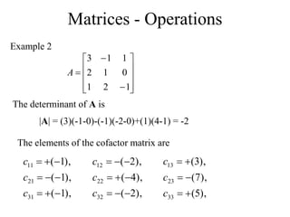
|A| = (3)(-1-0)-(-1)(-2-0)+(1)(4-1) = -2
),
1
(
),
1
(
),
1
(
31
21
11









c
c
c
The determinant of A is
The elements of the cofactor matrix are
),
2
(
),
4
(
),
2
(
32
22
12









c
c
c
),
5
(
),
7
(
),
3
(
33
23
13






c
c
c
Matrices - Operations















5
2
1
7
4
1
3
2
1
C
The cofactor matrix is therefore
so
















5
7
3
2
4
2
1
1
1
T
C
adjA
and


































5
.
2
5
.
3
5
.
1
0
.
1
0
.
2
0
.
1
5
.
0
5
.
0
5
.
0
5
7
3
2
4
2
1
1
1
2
1
1
A
adjA
A
Matrices - Operations
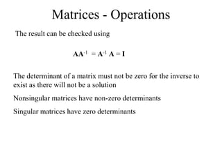
The result can be checked using
AA-1 = A-1 A = I
The determinant of a matrix must not be zero for the inverse to
exist as there will not be a solution
Nonsingular matrices have non-zero determinants
Singular matrices have zero determinants
Simple 2 x 2 case
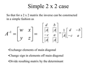
So that for a 2 x 2 matrix the inverse can be constructed
in a simple fashion as





















 a
c
b
d
A
A
a
A
c
A
b
A
d
1
•Exchange elements of main diagonal
•Change sign in elements off main diagonal
•Divide resulting matrix by the determinant









z
y
x
w
A 1
Simple 2 x 2 case
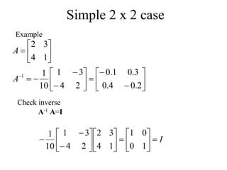
Example



























2
.
0
4
.
0
3
.
0
1
.
0
2
4
3
1
10
1
1
4
3
2
1
A
A
Check inverse
A-1 A=I
I























1
0
0
1
1
4
3
2
2
4
3
1
10
1
Ch5_51
5.1 Eigenvalues and Eigenvectors
Definition
Let A be an n  n matrix. A scalar  is called an eigenvalue of A
if there exists a nonzero vector x in Rn such that
Ax = x.
The vector x is called an eigenvector corresponding to .
Figure 5.1
Ch5_52
Computation of Eigenvalues and
Eigenvectors
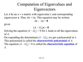
Let A be an n  n matrix with eigenvalue  and corresponding
eigenvector x. Thus Ax = x. This equation may be written
Ax – x = 0
given
(A – In)x = 0
Solving the equation |A – In| = 0 for  leads to all the eigenvalues
of A.
On expending the determinant |A – In|, we get a polynomial in .
This polynomial is called the characteristic polynomial of A.
The equation |A – In| = 0 is called the characteristic equation of
A.
Find the eigenvalues and eigenvectors of the matrix





 


5
3
6
4
A
Let us first derive the characteristic polynomial of A.
We get
Solution























 







5
3
6
4
1
0
0
1
5
3
6
4
2
I
A
2
18
)
5
)(
4
( 2
2 







 



I
A
We now solve the characteristic equation of A.
The eigenvalues of A are 2 and –1.
The corresponding eigenvectors are found by using these values
of  in the equation(A – I2)x = 0. There are many eigenvectors
corresponding to each eigenvalue.
1
or
2
0
)
1
)(
2
(
0
2
2









 




• For  = 2
We solve the equation (A – 2I2)x = 0 for x.
The matrix (A – 2I2) is obtained by subtracting 2 from the
diagonal elements of A. We get
0












 

2
1
3
3
6
6
x
x
This leads to the system of equations
giving x1 = –x2. The solutions to this system of equations are
x1 = –r, x2 = r, where r is a scalar. Thus the eigenvectors of A
corresponding to  = 2 are nonzero vectors of the form
0
3
3
0
6
6
2
1
2
1





x
x
x
x
1
1 2
2
1 1
v
1 1
x
x r
x
 
     
  
     
   
 
• For  = –1
We solve the equation (A + 1I2)x = 0 for x.
The matrix (A + 1I2) is obtained by adding 1 to the diagonal
elements of A. We get
0












 

2
1
6
3
6
3
x
x
This leads to the system of equations
Thus x1 = –2x2. The solutions to this system of equations are
x1 = –2s and x2 = s, where s is a scalar. Thus the eigenvectors
of A corresponding to  = –1 are nonzero vectors of the form
0
6
3
0
6
3
2
1
2
1





x
x
x
x
1
2 2
2
2 2
v
1 1
x
x s
x
 
     
  
     
   
 
Find the eigenvalues and eigenvectors of the matrix









2
2
2
2
5
4
2
4
5
A
The matrix A – I3 is obtained by subtracting  from
the diagonal elements of A.Thus
Solution

















2
2
2
2
5
4
2
4
5
3
I
A



















2
2
2
2
5
4
0
1
1
2
2
2
2
5
4
2
4
5
3
I
A
The characteristic polynomial of A is |A – I3|. Using row and
column operations to simplify determinants, we get
2
2
)
1
)(
10
(
)
1
)(
10
)(
1
(
]
10
11
)[
1
(
]
8
)
2
)(
9
)[(
1
(
2
4
2
2
9
4
0
0
1



































We now solving the characteristic equation of A:
The eigenvalues of A are 10 and 1.
The corresponding eigenvectors are found by using three values
of  in the equation (A – I3)x = 0.
10
,
1
0
)
1
)(
10
( 2








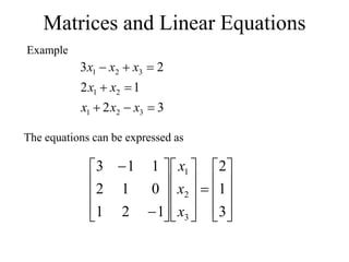
Matrices and Linear Equations
Example
3
2
1
2
2
3
3
2
1
2
1
3
2
1








x
x
x
x
x
x
x
x
The equations can be expressed as

































3
1
2
1
2
1
0
1
2
1
1
3
3
2
1
x
x
x
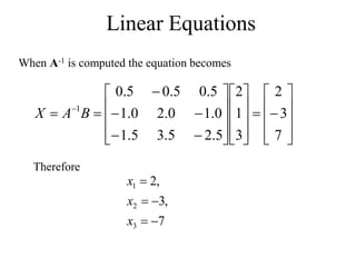
Linear Equations
When A-1 is computed the equation becomes






































 
7
3
2
3
1
2
5
.
2
5
.
3
5
.
1
0
.
1
0
.
2
0
.
1
5
.
0
5
.
0
5
.
0
1
B
A
X
Therefore
7
,
3
,
2
3
2
1





x
x
x
RANK OF A MATRIX
Let A be any m n matrix. Then A consists of n column
vectors a₁, a₂ ,....,a, which are m-vectors.
DEFINTION:
The rank of A is the maximal number of linearly
independent column vectors in A, i.e. the maximal
number of linearly independent vectors among {a₁,
a₂,......, a}.
If A = 0, then the rank of A is 0.
We write rk(A) for the rank of A. Note that we may
compute the rank of any matrix-square or not
Let us see how to compute 22 matrix:
EXAMPLE :
rk ( A)  2 if det  A  ad bc  0,since both columnvectors are
independent in this case.
The rank of a 22 matrix A =
 a b 
is given by
 c d 
 
rk(A) = 1 if det(A) = 0 but A  0 =
0 0
,since both column vectors
0 0
 
RANK OF 22 MATRIX
are not linearly independent, but there is a single column vector that is
linearly independent (i.e. non-zero).
rk(A) = 0 if A = 0
How do we compute rk(A) of m x n matrix?
EXAMPLE
Gauss elimination:
* Find the rank of a matrix
0 2
2 4
2 2
1 1

A= 0

2

0 1
 
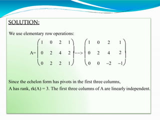
SOLUTION:
We use elementary row operations:
2 4 2 4
1 0 2 1  1 0 2 1 
A= 0 2  0 2 
   
0 2 2 1  0 0 2 1
Since the echelon form has pivots in the first three columns,
A has rank, rk(A) = 3. The first three columns of A are linearly independent.
EXAMPLE:
Find the rank of a matrix using normalform,
2 3 4 5 
3 4 5
5 6
10 11
6 
A=
4

7 

9 12

 
Solution:
Reduce the matrix to echelon form,
2 3 4 5  1 0 0 0
 4 5   1 2 
5 6 0 0
10 11 0 0
6     0
3
4 7  0
3
0

9 12
 
0 0

   
rank(A)=2

Matrices ,Basics, Determinant, Inverse, EigenValues, Linear Equations, RANK

  • 1.
  • 2.
    Matrices - Introduction Matrixalgebra has at least two advantages: •Reduces complicated systems of equations to simple expressions •Adaptable to systematic method of mathematical treatment and well suited to computers Definition: A matrix is a set or group of numbers arranged in a square or rectangular array enclosed by two brackets   1 1         0 3 2 4       d c b a
  • 3.
    Matrices - Introduction Properties: •Aspecified number of rows and a specified number of columns •Two numbers (rows x columns) describe the dimensions or size of the matrix. Examples: 3x3 matrix 2x4 matrix 1x2 matrix            3 3 3 5 1 4 4 2 1        2 3 3 3 0 1 0 1   1 1 
  • 4.
    Matrices - Introduction TYPESOF MATRICES 1. Column matrix or vector: The number of rows may be any integer but the number of columns is always 1           2 4 1       3 1             1 21 11 m a a a 
  • 5.
    Matrices - Introduction TYPESOF MATRICES 2. Row matrix or vector Any number of columns but only one row   6 1 1   2 5 3 0   n a a a a 1 13 12 11 
  • 6.
    Matrices - Introduction TYPESOF MATRICES 3. Rectangular matrix Contains more than one element and number of rows is not equal to the number of columns              6 7 7 7 7 3 1 1       0 3 3 0 2 0 0 1 1 1 n m
  • 7.
    Matrices - Introduction TYPESOF MATRICES 4. Square matrix The number of rows is equal to the number of columns (a square matrix A has an order of m)       0 3 1 1           1 6 6 0 9 9 1 1 1 m x m The principal or main diagonal of a square matrix is composed of all elements aij for which i=j
  • 8.
    Matrices - Introduction TYPESOF MATRICES 5. Diagonal matrix A square matrix where all the elements are zero except those on the main diagonal           1 0 0 0 2 0 0 0 1             9 0 0 0 0 5 0 0 0 0 3 0 0 0 0 3 i.e. aij =0 for all i = j aij = 0 for some or all i = j
  • 9.
    Matrices - Introduction TYPESOF MATRICES 6. Unit or Identity matrix - I A diagonal matrix with ones on the main diagonal             1 0 0 0 0 1 0 0 0 0 1 0 0 0 0 1       1 0 0 1 i.e. aij =0 for all i = j aij = 1 for some or all i = j       ij ij a a 0 0
  • 10.
    Matrices - Introduction TYPESOF MATRICES 7. Null (zero) matrix - 0 All elements in the matrix are zero           0 0 0           0 0 0 0 0 0 0 0 0 0  ij a For all i,j
  • 11.
    Matrices - Introduction TYPESOF MATRICES 8. Triangular matrix A square matrix whose elements above or below the main diagonal are all zero           3 2 5 0 1 2 0 0 1           3 2 5 0 1 2 0 0 1           3 0 0 6 1 0 9 8 1
  • 12.
    Matrices - Introduction TYPESOF MATRICES 8a. Upper triangular matrix A square matrix whose elements below the main diagonal are all zero i.e. aij = 0 for all i > j           3 0 0 8 1 0 7 8 1             3 0 0 0 8 7 0 0 4 7 1 0 4 4 7 1           ij ij ij ij ij ij a a a a a a 0 0 0
  • 13.
    Matrices - Introduction TYPESOF MATRICES A square matrix whose elements above the main diagonal are all zero 8b. Lower triangular matrix i.e. aij = 0 for all i < j           3 2 5 0 1 2 0 0 1           ij ij ij ij ij ij a a a a a a 0 0 0
  • 14.
    Matrices – Introduction TYPESOF MATRICES 9. Scalar matrix A diagonal matrix whose main diagonal elements are equal to the same scalar A scalar is defined as a single number or constant           1 0 0 0 1 0 0 0 1             6 0 0 0 0 6 0 0 0 0 6 0 0 0 0 6 i.e. aij = 0 for all i = j aij = a for all i = j           ij ij ij a a a 0 0 0 0 0 0
  • 15.
    Matrices - Operations EQUALITYOF MATRICES Two matrices are said to be equal only when all corresponding elements are equal Therefore their size or dimensions are equal as well           3 2 5 0 1 2 0 0 1           3 2 5 0 1 2 0 0 1 A = B = A = B
  • 16.
    Matrices - Operations Someproperties of equality: •IIf A = B, then B = A for all A and B •IIf A = B, and B = C, then A = C for all A, B and C           3 2 5 0 1 2 0 0 1 A = B =           33 32 31 23 22 21 13 12 11 b b b b b b b b b If A = B then ij ij b a 
  • 17.
    Matrices - Operations ADDITIONAND SUBTRACTION OF MATRICES The sum or difference of two matrices, A and B of the same size yields a matrix C of the same size ij ij ij b a c   Matrices of different sizes cannot be added or subtracted
  • 18.
    Matrices - Operations SCALARMULTIPLICATION OF MATRICES Matrices can be multiplied by a scalar (constant or single element) Let k be a scalar quantity; then kA = Ak Ex. If k=4 and                1 4 3 2 1 2 1 3 A
  • 19.
  • 20.
    Matrices - Operations MULTIPLICATIONOF MATRICES The product of two matrices is another matrix Two matrices A and B must be conformable for multiplication to be possible i.e. the number of columns of A must equal the number of rows of B Example. A x B = C (1x3) (3x1) (1x1)
  • 21.
    Matrices - Operations Bx A = Not possible! (2x1) (4x2) A x B = Not possible! (6x2) (6x3) Example A x B = C (2x3) (3x2) (2x2)
  • 22.
  • 23.
  • 24.
    Matrices - Operations Assumingthat matrices A, B and C are conformable for the operations indicated, the following are true: 1. AI = IA = A 2. A(BC) = (AB)C = ABC - (associative law) 3. A(B+C) = AB + AC - (first distributive law) 4. (A+B)C = AC + BC - (second distributive law) Caution! 1. AB not generally equal to BA, BA may not be conformable 2. If AB = 0, neither A nor B necessarily = 0 3. If AB = AC, B not necessarily = C
  • 25.
    Matrices - Operations IfAB = 0, neither A nor B necessarily = 0                      0 0 0 0 3 2 3 2 0 0 1 1
  • 26.
    Matrices - Operations Totranspose: Interchange rows and columns The dimensions of AT are the reverse of the dimensions of A         1 3 5 7 4 2 3 2A A             1 7 3 4 5 2 2 3 T T A A 2 x 3 3 x 2
  • 27.
    Matrices - Operations Propertiesof transposed matrices: 1. (A+B)T = AT + BT 2. (AB)T = BT AT 3. (kA)T = kAT 4. (AT)T = A
  • 28.
    Matrices - Operations SYMMETRICMATRICES A Square matrix is symmetric if it is equal to its transpose: A = AT               d b b a A d b b a A T
  • 29.
    Matrices - Operations DETERMINANTOF A MATRIX To compute the inverse of a matrix, the determinant is required Each square matrix A has a unit scalar value called the determinant of A, denoted by det A or |A| 5 6 2 1 5 6 2 1         A A If then
  • 30.
    Matrices - Operations IfA = [A] is a single element (1x1), then the determinant is defined as the value of the element Then |A| =det A = a11 If A is (n x n), its determinant may be defined in terms of order (n-1) or less.
  • 31.
    Matrices - Operations MINORS IfA is an n x n matrix and one row and one column are deleted, the resulting matrix is an (n-1) x (n-1) submatrix of A. The determinant of such a submatrix is called a minor of A and is designated by mij , where i and j correspond to the deleted row and column, respectively. mij is the minor of the element aij in A.
  • 32.
    Matrices - Operations            33 32 31 23 22 21 13 12 11 a a a a a a a a a A Eachelement in A has a minor Delete first row and column from A . The determinant of the remaining 2 x 2 submatrix is the minor of a11 eg. 33 32 23 22 11 a a a a m 
  • 33.
    Matrices - Operations Thereforethe minor of a12 is: And the minor for a13 is: 33 31 23 21 12 a a a a m  32 31 22 21 13 a a a a m 
  • 34.
    Matrices - Operations COFACTORS Thecofactor Cij of an element aij is defined as: ij j i ij m C    ) 1 ( When the sum of a row number i and column j is even, cij = mij and when i+j is odd, cij =-mij 13 13 3 1 13 12 12 2 1 12 11 11 1 1 11 ) 1 ( ) 3 , 1 ( ) 1 ( ) 2 , 1 ( ) 1 ( ) 1 , 1 ( m m j i c m m j i c m m j i c                     
  • 35.
    Matrices - Operations DETERMINANTSCONTINUED The determinant of an n x n matrix A can now be defined as n nc a c a c a A A 1 1 12 12 11 11 det       The determinant of A is therefore the sum of the products of the elements of the first row of A and their corresponding cofactors. (It is possible to define |A| in terms of any other row or column but for simplicity, the first row only is used)
  • 36.
    Matrices - Operations Thereforethe 2 x 2 matrix :        22 21 12 11 a a a a A Has cofactors : 22 22 11 11 a a m c    And: 21 21 12 12 a a m c       And the determinant of A is: 21 12 22 11 12 12 11 11 a a a a c a c a A    
  • 37.
    Matrices - Operations Example1:        2 1 1 3 A 5 ) 1 )( 1 ( ) 2 )( 3 (    A
  • 38.
    Matrices - Operations Fora 3 x 3 matrix:            33 32 31 23 22 21 13 12 11 a a a a a a a a a A The cofactors of the first row are: 31 22 32 21 32 31 22 21 13 31 23 33 21 33 31 23 21 12 32 23 33 22 33 32 23 22 11 ) ( a a a a a a a a c a a a a a a a a c a a a a a a a a c           
  • 39.
    Matrices - Operations Thedeterminant of a matrix A is: 21 12 22 11 12 12 11 11 a a a a c a c a A     Which by substituting for the cofactors in this case is: ) ( ) ( ) ( 31 22 32 21 13 31 23 33 21 12 32 23 33 22 11 a a a a a a a a a a a a a a a A      
  • 40.
    Matrices - Operations Example2:             1 0 1 3 2 0 1 0 1 A 4 ) 2 0 )( 1 ( ) 3 0 )( 0 ( ) 0 2 )( 1 (        A ) ( ) ( ) ( 31 22 32 21 13 31 23 33 21 12 32 23 33 22 11 a a a a a a a a a a a a a a a A      
  • 41.
    Matrices - Operations ADJOINTMATRICES A cofactor matrix C of a matrix A is the square matrix of the same order as A in which each element aij is replaced by its cofactor cij . Example:         4 3 2 1 A         1 2 3 4 C If The cofactor C of A is
  • 42.
    Matrices - Operations Theadjoint matrix of A, denoted by adj A, is the transpose of its cofactor matrix T C adjA  It can be shown that: A(adj A) = (adjA) A = |A| I Example:                      1 3 2 4 10 ) 3 )( 2 ( ) 4 )( 1 ( 4 3 2 1 T C adjA A A
  • 43.
    Matrices - Operations I adjA A10 10 0 0 10 1 3 2 4 4 3 2 1 ) (                        I A adjA 10 10 0 0 10 4 3 2 1 1 3 2 4 ) (                       
  • 44.
    Matrices - Operations USINGTHE ADJOINT MATRIX IN MATRIX INVERSION A adjA A  1 Since AA-1 = A-1 A = I and A(adj A) = (adjA) A = |A| I then
  • 45.
    Matrices - Operations Example                 1 . 0 3 . 0 2 . 0 4 . 0 1 3 2 4 10 1 1 A        4 3 2 1 A = To check AA-1 = A-1 A = I I A A I AA                                                 1 0 0 1 4 3 2 1 1 . 0 3 . 0 2 . 0 4 . 0 1 0 0 1 1 . 0 3 . 0 2 . 0 4 . 0 4 3 2 1 1 1
  • 46.
    Matrices - Operations Example2              1 2 1 0 1 2 1 1 3 A |A| = (3)(-1-0)-(-1)(-2-0)+(1)(4-1) = -2 ), 1 ( ), 1 ( ), 1 ( 31 21 11          c c c The determinant of A is The elements of the cofactor matrix are ), 2 ( ), 4 ( ), 2 ( 32 22 12          c c c ), 5 ( ), 7 ( ), 3 ( 33 23 13       c c c
  • 47.
    Matrices - Operations                5 2 1 7 4 1 3 2 1 C Thecofactor matrix is therefore so                 5 7 3 2 4 2 1 1 1 T C adjA and                                   5 . 2 5 . 3 5 . 1 0 . 1 0 . 2 0 . 1 5 . 0 5 . 0 5 . 0 5 7 3 2 4 2 1 1 1 2 1 1 A adjA A
  • 48.
    Matrices - Operations Theresult can be checked using AA-1 = A-1 A = I The determinant of a matrix must not be zero for the inverse to exist as there will not be a solution Nonsingular matrices have non-zero determinants Singular matrices have zero determinants
  • 49.
    Simple 2 x2 case So that for a 2 x 2 matrix the inverse can be constructed in a simple fashion as                       a c b d A A a A c A b A d 1 •Exchange elements of main diagonal •Change sign in elements off main diagonal •Divide resulting matrix by the determinant          z y x w A 1
  • 50.
    Simple 2 x2 case Example                            2 . 0 4 . 0 3 . 0 1 . 0 2 4 3 1 10 1 1 4 3 2 1 A A Check inverse A-1 A=I I                        1 0 0 1 1 4 3 2 2 4 3 1 10 1
  • 51.
    Ch5_51 5.1 Eigenvalues andEigenvectors Definition Let A be an n  n matrix. A scalar  is called an eigenvalue of A if there exists a nonzero vector x in Rn such that Ax = x. The vector x is called an eigenvector corresponding to . Figure 5.1
  • 52.
    Ch5_52 Computation of Eigenvaluesand Eigenvectors Let A be an n  n matrix with eigenvalue  and corresponding eigenvector x. Thus Ax = x. This equation may be written Ax – x = 0 given (A – In)x = 0 Solving the equation |A – In| = 0 for  leads to all the eigenvalues of A. On expending the determinant |A – In|, we get a polynomial in . This polynomial is called the characteristic polynomial of A. The equation |A – In| = 0 is called the characteristic equation of A.
  • 53.
    Find the eigenvaluesand eigenvectors of the matrix          5 3 6 4 A Let us first derive the characteristic polynomial of A. We get Solution                                 5 3 6 4 1 0 0 1 5 3 6 4 2 I A 2 18 ) 5 )( 4 ( 2 2              I A We now solve the characteristic equation of A. The eigenvalues of A are 2 and –1. The corresponding eigenvectors are found by using these values of  in the equation(A – I2)x = 0. There are many eigenvectors corresponding to each eigenvalue. 1 or 2 0 ) 1 )( 2 ( 0 2 2               
  • 54.
    • For = 2 We solve the equation (A – 2I2)x = 0 for x. The matrix (A – 2I2) is obtained by subtracting 2 from the diagonal elements of A. We get 0                2 1 3 3 6 6 x x This leads to the system of equations giving x1 = –x2. The solutions to this system of equations are x1 = –r, x2 = r, where r is a scalar. Thus the eigenvectors of A corresponding to  = 2 are nonzero vectors of the form 0 3 3 0 6 6 2 1 2 1      x x x x 1 1 2 2 1 1 v 1 1 x x r x                       
  • 55.
    • For = –1 We solve the equation (A + 1I2)x = 0 for x. The matrix (A + 1I2) is obtained by adding 1 to the diagonal elements of A. We get 0                2 1 6 3 6 3 x x This leads to the system of equations Thus x1 = –2x2. The solutions to this system of equations are x1 = –2s and x2 = s, where s is a scalar. Thus the eigenvectors of A corresponding to  = –1 are nonzero vectors of the form 0 6 3 0 6 3 2 1 2 1      x x x x 1 2 2 2 2 2 v 1 1 x x s x                       
  • 56.
    Find the eigenvaluesand eigenvectors of the matrix          2 2 2 2 5 4 2 4 5 A The matrix A – I3 is obtained by subtracting  from the diagonal elements of A.Thus Solution                  2 2 2 2 5 4 2 4 5 3 I A                    2 2 2 2 5 4 0 1 1 2 2 2 2 5 4 2 4 5 3 I A The characteristic polynomial of A is |A – I3|. Using row and column operations to simplify determinants, we get
  • 57.
    2 2 ) 1 )( 10 ( ) 1 )( 10 )( 1 ( ] 10 11 )[ 1 ( ] 8 ) 2 )( 9 )[( 1 ( 2 4 2 2 9 4 0 0 1                                    We now solvingthe characteristic equation of A: The eigenvalues of A are 10 and 1. The corresponding eigenvectors are found by using three values of  in the equation (A – I3)x = 0. 10 , 1 0 ) 1 )( 10 ( 2        
  • 58.
    Matrices and LinearEquations Example 3 2 1 2 2 3 3 2 1 2 1 3 2 1         x x x x x x x x The equations can be expressed as                                  3 1 2 1 2 1 0 1 2 1 1 3 3 2 1 x x x
  • 59.
    Linear Equations When A-1is computed the equation becomes                                         7 3 2 3 1 2 5 . 2 5 . 3 5 . 1 0 . 1 0 . 2 0 . 1 5 . 0 5 . 0 5 . 0 1 B A X Therefore 7 , 3 , 2 3 2 1      x x x
  • 60.
    RANK OF AMATRIX Let A be any m n matrix. Then A consists of n column vectors a₁, a₂ ,....,a, which are m-vectors. DEFINTION: The rank of A is the maximal number of linearly independent column vectors in A, i.e. the maximal number of linearly independent vectors among {a₁, a₂,......, a}. If A = 0, then the rank of A is 0. We write rk(A) for the rank of A. Note that we may compute the rank of any matrix-square or not
  • 61.
    Let us seehow to compute 22 matrix: EXAMPLE : rk ( A)  2 if det  A  ad bc  0,since both columnvectors are independent in this case. The rank of a 22 matrix A =  a b  is given by  c d    rk(A) = 1 if det(A) = 0 but A  0 = 0 0 ,since both column vectors 0 0   RANK OF 22 MATRIX are not linearly independent, but there is a single column vector that is linearly independent (i.e. non-zero). rk(A) = 0 if A = 0 How do we compute rk(A) of m x n matrix?
  • 62.
    EXAMPLE Gauss elimination: * Findthe rank of a matrix 0 2 2 4 2 2 1 1  A= 0  2  0 1  
  • 63.
    SOLUTION: We use elementaryrow operations: 2 4 2 4 1 0 2 1  1 0 2 1  A= 0 2  0 2      0 2 2 1  0 0 2 1 Since the echelon form has pivots in the first three columns, A has rank, rk(A) = 3. The first three columns of A are linearly independent.
  • 64.
    EXAMPLE: Find the rankof a matrix using normalform, 2 3 4 5  3 4 5 5 6 10 11 6  A= 4  7   9 12    Solution: Reduce the matrix to echelon form, 2 3 4 5  1 0 0 0  4 5   1 2  5 6 0 0 10 11 0 0 6     0 3 4 7  0 3 0  9 12   0 0      rank(A)=2