Download as PDF, PPTX


![Images/
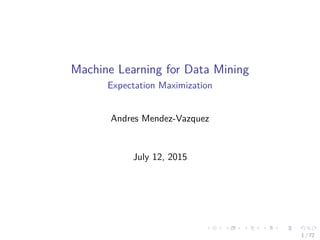
The function we would like to have
The Q function
We want an estimation of the complete-data log-likelihood
log p (X, Y|Θ) (15)
Based in the info provided by X, Θn−1 where Θn−1 is a previously
estimated set of parameters at step n.
Think about the following, if we want to remove Y
ˆ
[log p (X, Y|Θ)] p (Y|X, Θn−1) dY (16)
Remark: We integrate out Y - Actually, this is the expected value of
log p (X, Y|Θ).
23 / 126](https://image.slidesharecdn.com/04-151212035340/85/07-Machine-Learning-Expectation-Maximization-49-320.jpg)
![Images/
The function we would like to have
The Q function
We want an estimation of the complete-data log-likelihood
log p (X, Y|Θ) (15)
Based in the info provided by X, Θn−1 where Θn−1 is a previously
estimated set of parameters at step n.
Think about the following, if we want to remove Y
ˆ
[log p (X, Y|Θ)] p (Y|X, Θn−1) dY (16)
Remark: We integrate out Y - Actually, this is the expected value of
log p (X, Y|Θ).
23 / 126](https://image.slidesharecdn.com/04-151212035340/85/07-Machine-Learning-Expectation-Maximization-50-320.jpg)

![Images/
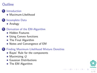
Use the Expected Value
Then, we want an iterative method to guess Θ from Θn−1
Q (Θ, Θn−1) = E [log p (X, Y|Θ) |X, Θn−1] (17)
Take in account that
1 X, Θn−1 are taken as constants.
2 Θ is a normal variable that we wish to adjust.
3 Y is a random variable governed by distribution
p (Y|X, Θn−1)=marginal distribution of missing data.
25 / 126](https://image.slidesharecdn.com/04-151212035340/85/07-Machine-Learning-Expectation-Maximization-52-320.jpg)
![Images/
Use the Expected Value
Then, we want an iterative method to guess Θ from Θn−1
Q (Θ, Θn−1) = E [log p (X, Y|Θ) |X, Θn−1] (17)
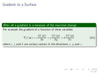
Take in account that
1 X, Θn−1 are taken as constants.
2 Θ is a normal variable that we wish to adjust.
3 Y is a random variable governed by distribution
p (Y|X, Θn−1)=marginal distribution of missing data.
25 / 126](https://image.slidesharecdn.com/04-151212035340/85/07-Machine-Learning-Expectation-Maximization-53-320.jpg)
![Images/
Use the Expected Value
Then, we want an iterative method to guess Θ from Θn−1
Q (Θ, Θn−1) = E [log p (X, Y|Θ) |X, Θn−1] (17)
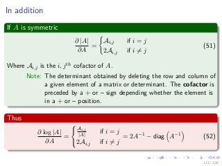
Take in account that
1 X, Θn−1 are taken as constants.
2 Θ is a normal variable that we wish to adjust.
3 Y is a random variable governed by distribution
p (Y|X, Θn−1)=marginal distribution of missing data.
25 / 126](https://image.slidesharecdn.com/04-151212035340/85/07-Machine-Learning-Expectation-Maximization-54-320.jpg)
![Images/
Use the Expected Value
Then, we want an iterative method to guess Θ from Θn−1
Q (Θ, Θn−1) = E [log p (X, Y|Θ) |X, Θn−1] (17)
Take in account that
1 X, Θn−1 are taken as constants.
2 Θ is a normal variable that we wish to adjust.
3 Y is a random variable governed by distribution
p (Y|X, Θn−1)=marginal distribution of missing data.
25 / 126](https://image.slidesharecdn.com/04-151212035340/85/07-Machine-Learning-Expectation-Maximization-55-320.jpg)
![Images/
Another Interpretation
Given the previous information
E [log p (X, Y|Θ) |X, Θn−1] =
´
Y∈Y log p (X, Y|Θ) p (Y|X, Θn−1) dY
Something Notable
1 In the best of cases, this marginal distribution is a simple analytical
expression of the assumed parameter Θn−1.
2 In the worst of cases, this density might be very hard to obtain.
Actually, we use
p (Y, X|Θn−1) = p (Y|X, Θn−1) p (X|Θn−1) (18)
which is not dependent on Θ.
26 / 126](https://image.slidesharecdn.com/04-151212035340/85/07-Machine-Learning-Expectation-Maximization-56-320.jpg)
![Images/
Another Interpretation
Given the previous information
E [log p (X, Y|Θ) |X, Θn−1] =
´
Y∈Y log p (X, Y|Θ) p (Y|X, Θn−1) dY
Something Notable
1 In the best of cases, this marginal distribution is a simple analytical
expression of the assumed parameter Θn−1.
2 In the worst of cases, this density might be very hard to obtain.
Actually, we use
p (Y, X|Θn−1) = p (Y|X, Θn−1) p (X|Θn−1) (18)
which is not dependent on Θ.
26 / 126](https://image.slidesharecdn.com/04-151212035340/85/07-Machine-Learning-Expectation-Maximization-57-320.jpg)
![Images/
Another Interpretation
Given the previous information
E [log p (X, Y|Θ) |X, Θn−1] =
´
Y∈Y log p (X, Y|Θ) p (Y|X, Θn−1) dY
Something Notable
1 In the best of cases, this marginal distribution is a simple analytical
expression of the assumed parameter Θn−1.
2 In the worst of cases, this density might be very hard to obtain.
Actually, we use
p (Y, X|Θn−1) = p (Y|X, Θn−1) p (X|Θn−1) (18)
which is not dependent on Θ.
26 / 126](https://image.slidesharecdn.com/04-151212035340/85/07-Machine-Learning-Expectation-Maximization-58-320.jpg)
![Images/
Another Interpretation
Given the previous information
E [log p (X, Y|Θ) |X, Θn−1] =
´
Y∈Y log p (X, Y|Θ) p (Y|X, Θn−1) dY
Something Notable
1 In the best of cases, this marginal distribution is a simple analytical
expression of the assumed parameter Θn−1.
2 In the worst of cases, this density might be very hard to obtain.
Actually, we use
p (Y, X|Θn−1) = p (Y|X, Θn−1) p (X|Θn−1) (18)
which is not dependent on Θ.
26 / 126](https://image.slidesharecdn.com/04-151212035340/85/07-Machine-Learning-Expectation-Maximization-59-320.jpg)

![Images/
Back to the Q function
The intuition
We have the following analogy:
Consider h (θ, Y ) a function
θ a constant
Y ∼ pY (y), a random variable with distribution pY (y).
Thus, if Y is a discrete random variable
q (θ) = EY [h (θ, Y )] =
y
h (θ, y) pY (y) (19)
28 / 126](https://image.slidesharecdn.com/04-151212035340/85/07-Machine-Learning-Expectation-Maximization-61-320.jpg)
![Images/
Back to the Q function
The intuition
We have the following analogy:
Consider h (θ, Y ) a function
θ a constant
Y ∼ pY (y), a random variable with distribution pY (y).
Thus, if Y is a discrete random variable
q (θ) = EY [h (θ, Y )] =
y
h (θ, y) pY (y) (19)
28 / 126](https://image.slidesharecdn.com/04-151212035340/85/07-Machine-Learning-Expectation-Maximization-62-320.jpg)
![Images/
Back to the Q function
The intuition
We have the following analogy:
Consider h (θ, Y ) a function
θ a constant
Y ∼ pY (y), a random variable with distribution pY (y).
Thus, if Y is a discrete random variable
q (θ) = EY [h (θ, Y )] =
y
h (θ, y) pY (y) (19)
28 / 126](https://image.slidesharecdn.com/04-151212035340/85/07-Machine-Learning-Expectation-Maximization-63-320.jpg)
![Images/
Back to the Q function
The intuition
We have the following analogy:
Consider h (θ, Y ) a function
θ a constant
Y ∼ pY (y), a random variable with distribution pY (y).
Thus, if Y is a discrete random variable
q (θ) = EY [h (θ, Y )] =
y
h (θ, y) pY (y) (19)
28 / 126](https://image.slidesharecdn.com/04-151212035340/85/07-Machine-Learning-Expectation-Maximization-64-320.jpg)
![Images/
Back to the Q function
The intuition
We have the following analogy:
Consider h (θ, Y ) a function
θ a constant
Y ∼ pY (y), a random variable with distribution pY (y).
Thus, if Y is a discrete random variable
q (θ) = EY [h (θ, Y )] =
y
h (θ, y) pY (y) (19)
28 / 126](https://image.slidesharecdn.com/04-151212035340/85/07-Machine-Learning-Expectation-Maximization-65-320.jpg)


![Images/
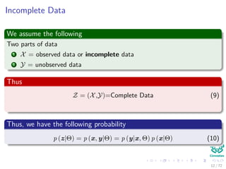
Thus
Then
θn+1 =argmaxΘ
y
P (y|X, Θn) ln
P (X, y, Θ)
P (y, Θ)
P (y, Θ)
P (Θ)
=argmaxΘ
y
P (y|X, Θn) ln
P (X, y, Θ)
P (Θ)
=argmaxΘ
y
P (y|X, Θn) ln (P (X, y|Θ))
=argmaxΘ Ey|X,Θn
[ln (P (X, y|Θ))]
Then argmaxΘ {l (Θ|Θn)} ≈ argmaxΘ Ey|X,Θn
[ln (P (X, y|Θ))]
52 / 126](https://image.slidesharecdn.com/04-151212035340/85/07-Machine-Learning-Expectation-Maximization-126-320.jpg)
![Images/
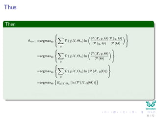
Thus
Then
θn+1 =argmaxΘ
y
P (y|X, Θn) ln
P (X, y, Θ)
P (y, Θ)
P (y, Θ)
P (Θ)
=argmaxΘ
y
P (y|X, Θn) ln
P (X, y, Θ)
P (Θ)
=argmaxΘ
y
P (y|X, Θn) ln (P (X, y|Θ))
=argmaxΘ Ey|X,Θn
[ln (P (X, y|Θ))]
Then argmaxΘ {l (Θ|Θn)} ≈ argmaxΘ Ey|X,Θn
[ln (P (X, y|Θ))]
52 / 126](https://image.slidesharecdn.com/04-151212035340/85/07-Machine-Learning-Expectation-Maximization-127-320.jpg)
![Images/
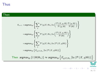
Thus
Then
θn+1 =argmaxΘ
y
P (y|X, Θn) ln
P (X, y, Θ)
P (y, Θ)
P (y, Θ)
P (Θ)
=argmaxΘ
y
P (y|X, Θn) ln
P (X, y, Θ)
P (Θ)
=argmaxΘ
y
P (y|X, Θn) ln (P (X, y|Θ))
=argmaxΘ Ey|X,Θn
[ln (P (X, y|Θ))]
Then argmaxΘ {l (Θ|Θn)} ≈ argmaxΘ Ey|X,Θn
[ln (P (X, y|Θ))]
52 / 126](https://image.slidesharecdn.com/04-151212035340/85/07-Machine-Learning-Expectation-Maximization-128-320.jpg)
![Images/
Thus
Then
θn+1 =argmaxΘ
y
P (y|X, Θn) ln
P (X, y, Θ)
P (y, Θ)
P (y, Θ)
P (Θ)
=argmaxΘ
y
P (y|X, Θn) ln
P (X, y, Θ)
P (Θ)
=argmaxΘ
y
P (y|X, Θn) ln (P (X, y|Θ))
=argmaxΘ Ey|X,Θn
[ln (P (X, y|Θ))]
Then argmaxΘ {l (Θ|Θn)} ≈ argmaxΘ Ey|X,Θn
[ln (P (X, y|Θ))]
52 / 126](https://image.slidesharecdn.com/04-151212035340/85/07-Machine-Learning-Expectation-Maximization-129-320.jpg)
![Images/
Thus
Then
θn+1 =argmaxΘ
y
P (y|X, Θn) ln
P (X, y, Θ)
P (y, Θ)
P (y, Θ)
P (Θ)
=argmaxΘ
y
P (y|X, Θn) ln
P (X, y, Θ)
P (Θ)
=argmaxΘ
y
P (y|X, Θn) ln (P (X, y|Θ))
=argmaxΘ Ey|X,Θn
[ln (P (X, y|Θ))]
Then argmaxΘ {l (Θ|Θn)} ≈ argmaxΘ Ey|X,Θn
[ln (P (X, y|Θ))]
52 / 126](https://image.slidesharecdn.com/04-151212035340/85/07-Machine-Learning-Expectation-Maximization-130-320.jpg)

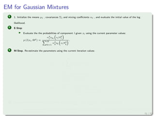
![Images/
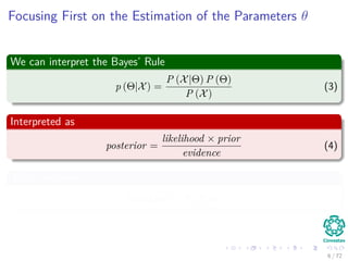
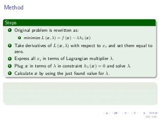
The EM-Algorithm
Steps of EM
1 Expectation under hidden variables.
2 Maximization of the resulting formula.
E-Step
Determine the conditional expectation, Ey|X,Θn
[ln (P (X, y|Θ))].
M-Step
Maximize this expression with respect to Θ.
54 / 126](https://image.slidesharecdn.com/04-151212035340/85/07-Machine-Learning-Expectation-Maximization-132-320.jpg)
![Images/
The EM-Algorithm
Steps of EM
1 Expectation under hidden variables.
2 Maximization of the resulting formula.
E-Step
Determine the conditional expectation, Ey|X,Θn
[ln (P (X, y|Θ))].
M-Step
Maximize this expression with respect to Θ.
54 / 126](https://image.slidesharecdn.com/04-151212035340/85/07-Machine-Learning-Expectation-Maximization-133-320.jpg)
![Images/
The EM-Algorithm
Steps of EM
1 Expectation under hidden variables.
2 Maximization of the resulting formula.
E-Step
Determine the conditional expectation, Ey|X,Θn
[ln (P (X, y|Θ))].
M-Step
Maximize this expression with respect to Θ.
54 / 126](https://image.slidesharecdn.com/04-151212035340/85/07-Machine-Learning-Expectation-Maximization-134-320.jpg)
![Images/
The EM-Algorithm
Steps of EM
1 Expectation under hidden variables.
2 Maximization of the resulting formula.
E-Step
Determine the conditional expectation, Ey|X,Θn
[ln (P (X, y|Θ))].
M-Step
Maximize this expression with respect to Θ.
54 / 126](https://image.slidesharecdn.com/04-151212035340/85/07-Machine-Learning-Expectation-Maximization-135-320.jpg)


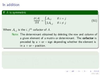
![Images/
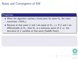
Notes and Convergence of EM
Properties
When the algorithm reaches a fixed point for some Θn, the value
maximizes l (Θ|Θn).
Definition
A fixed point of a function is an element on domain that is mapped to
itself by the function:
f (x) = x
Basically the EM algorithm does the following
EM [Θ∗
] = Θ∗
58 / 126](https://image.slidesharecdn.com/04-151212035340/85/07-Machine-Learning-Expectation-Maximization-143-320.jpg)
![Images/
Notes and Convergence of EM
Properties
When the algorithm reaches a fixed point for some Θn, the value
maximizes l (Θ|Θn).
Definition
A fixed point of a function is an element on domain that is mapped to
itself by the function:
f (x) = x
Basically the EM algorithm does the following
EM [Θ∗
] = Θ∗
58 / 126](https://image.slidesharecdn.com/04-151212035340/85/07-Machine-Learning-Expectation-Maximization-144-320.jpg)
![Images/
Notes and Convergence of EM
Properties
When the algorithm reaches a fixed point for some Θn, the value
maximizes l (Θ|Θn).
Definition
A fixed point of a function is an element on domain that is mapped to
itself by the function:
f (x) = x
Basically the EM algorithm does the following
EM [Θ∗
] = Θ∗
58 / 126](https://image.slidesharecdn.com/04-151212035340/85/07-Machine-Learning-Expectation-Maximization-145-320.jpg)


![Images/
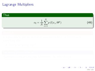
Now
We have
log L (Θ|X, Y) = log [P (X, Y|Θ)] (30)
Remember that X = {x1, x2, ..., xN } with Y = {y1, y2, ..., yN } and
assuming independence
log [P (X, Y|Θ)] = log [P (x1, x2, ..., xN , y1, y2, ..., yN |Θ)]
= log [P (x1, y1, ..., xi, yi, ..., xN , yN |Θ)]
= log
N
i=1
P (xi, yi|Θ)
=
N
i=1
log P (xi, yi|Θ)
66 / 126](https://image.slidesharecdn.com/04-151212035340/85/07-Machine-Learning-Expectation-Maximization-161-320.jpg)
![Images/
Now
We have
log L (Θ|X, Y) = log [P (X, Y|Θ)] (30)
Remember that X = {x1, x2, ..., xN } with Y = {y1, y2, ..., yN } and
assuming independence
log [P (X, Y|Θ)] = log [P (x1, x2, ..., xN , y1, y2, ..., yN |Θ)]
= log [P (x1, y1, ..., xi, yi, ..., xN , yN |Θ)]
= log
N
i=1
P (xi, yi|Θ)
=
N
i=1
log P (xi, yi|Θ)
66 / 126](https://image.slidesharecdn.com/04-151212035340/85/07-Machine-Learning-Expectation-Maximization-162-320.jpg)
![Images/
Now
We have
log L (Θ|X, Y) = log [P (X, Y|Θ)] (30)
Remember that X = {x1, x2, ..., xN } with Y = {y1, y2, ..., yN } and
assuming independence
log [P (X, Y|Θ)] = log [P (x1, x2, ..., xN , y1, y2, ..., yN |Θ)]
= log [P (x1, y1, ..., xi, yi, ..., xN , yN |Θ)]
= log
N
i=1
P (xi, yi|Θ)
=
N
i=1
log P (xi, yi|Θ)
66 / 126](https://image.slidesharecdn.com/04-151212035340/85/07-Machine-Learning-Expectation-Maximization-163-320.jpg)
![Images/
Now
We have
log L (Θ|X, Y) = log [P (X, Y|Θ)] (30)
Remember that X = {x1, x2, ..., xN } with Y = {y1, y2, ..., yN } and
assuming independence
log [P (X, Y|Θ)] = log [P (x1, x2, ..., xN , y1, y2, ..., yN |Θ)]
= log [P (x1, y1, ..., xi, yi, ..., xN , yN |Θ)]
= log
N
i=1
P (xi, yi|Θ)
=
N
i=1
log P (xi, yi|Θ)
66 / 126](https://image.slidesharecdn.com/04-151212035340/85/07-Machine-Learning-Expectation-Maximization-164-320.jpg)
![Images/
Now
We have
log L (Θ|X, Y) = log [P (X, Y|Θ)] (30)
Remember that X = {x1, x2, ..., xN } with Y = {y1, y2, ..., yN } and
assuming independence
log [P (X, Y|Θ)] = log [P (x1, x2, ..., xN , y1, y2, ..., yN |Θ)]
= log [P (x1, y1, ..., xi, yi, ..., xN , yN |Θ)]
= log
N
i=1
P (xi, yi|Θ)
=
N
i=1
log P (xi, yi|Θ)
66 / 126](https://image.slidesharecdn.com/04-151212035340/85/07-Machine-Learning-Expectation-Maximization-165-320.jpg)
![Images/
Then
Thus, by the chain Rule
N
i=1
log P (xi, yi|Θ) =
N
i=1
log [P (xi|yi, θyi ) P (yi|θyi )] (31)
Question Do you need yi if you know θyi or the other way around?
Finally
N
i=1
log [P (xi|yi, θyi ) P (yi|θyi )] =
N
i=1
log [P (yi) pyi (xi|θyi )] (32)
NOPE: You do not need yi if you know θyi or the other way around.
67 / 126](https://image.slidesharecdn.com/04-151212035340/85/07-Machine-Learning-Expectation-Maximization-166-320.jpg)
![Images/
Then
Thus, by the chain Rule
N
i=1
log P (xi, yi|Θ) =
N
i=1
log [P (xi|yi, θyi ) P (yi|θyi )] (31)
Question Do you need yi if you know θyi or the other way around?
Finally
N
i=1
log [P (xi|yi, θyi ) P (yi|θyi )] =
N
i=1
log [P (yi) pyi (xi|θyi )] (32)
NOPE: You do not need yi if you know θyi or the other way around.
67 / 126](https://image.slidesharecdn.com/04-151212035340/85/07-Machine-Learning-Expectation-Maximization-167-320.jpg)
![Images/
Finally, we have
Making αyi
= P (yi)
log L (Θ|X, Y) =
N
i=1
log [αyi P (xi|yi, θyi )] (33)
68 / 126](https://image.slidesharecdn.com/04-151212035340/85/07-Machine-Learning-Expectation-Maximization-168-320.jpg)


![Images/
Now, using equation 17
Then
Q (Θ|Θg
) =
y∈Y
log (L (Θ|X, y)) p (y|X, Θg
)
=
y∈Y
N
i=1
log [αyi pyi (xi|θyi )]
N
j=1
p (yj|xj, Θg
)
78 / 126](https://image.slidesharecdn.com/04-151212035340/85/07-Machine-Learning-Expectation-Maximization-187-320.jpg)
![Images/
Now, using equation 17
Then
Q (Θ|Θg
) =
y∈Y
log (L (Θ|X, y)) p (y|X, Θg
)
=
y∈Y
N
i=1
log [αyi pyi (xi|θyi )]
N
j=1
p (yj|xj, Θg
)
78 / 126](https://image.slidesharecdn.com/04-151212035340/85/07-Machine-Learning-Expectation-Maximization-188-320.jpg)


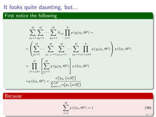
![Images/
Then
We have
Q (Θ|Θg
) =
M
y1=1
M
y2=1
· · ·
M
yN =1
N
i=1
log [αyi pyi (xi|θyi )]
N
j=1
p (yj|xj, Θg
)
80 / 126](https://image.slidesharecdn.com/04-151212035340/85/07-Machine-Learning-Expectation-Maximization-191-320.jpg)
![Images/
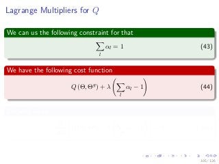
We introduce the following
We have the following function
δl,yi
=
1 I = yi
0 I = yi
Therefore, we can do the following
αi =
M
j=1
δi,jαj
Then
log [αyi pyi (xi|θyi )]
N
j=1
p (yj|xj, Θg
) =
M
l=1
δl,yi log [αlpl (xi|θl)]
N
j=1
p (yj|xj, Θg
)
81 / 126](https://image.slidesharecdn.com/04-151212035340/85/07-Machine-Learning-Expectation-Maximization-192-320.jpg)
![Images/
We introduce the following
We have the following function
δl,yi
=
1 I = yi
0 I = yi
Therefore, we can do the following
αi =
M
j=1
δi,jαj
Then
log [αyi pyi (xi|θyi )]
N
j=1
p (yj|xj, Θg
) =
M
l=1
δl,yi log [αlpl (xi|θl)]
N
j=1
p (yj|xj, Θg
)
81 / 126](https://image.slidesharecdn.com/04-151212035340/85/07-Machine-Learning-Expectation-Maximization-193-320.jpg)
![Images/
We introduce the following
We have the following function
δl,yi
=
1 I = yi
0 I = yi
Therefore, we can do the following
αi =
M
j=1
δi,jαj
Then
log [αyi pyi (xi|θyi )]
N
j=1
p (yj|xj, Θg
) =
M
l=1
δl,yi log [αlpl (xi|θl)]
N
j=1
p (yj|xj, Θg
)
81 / 126](https://image.slidesharecdn.com/04-151212035340/85/07-Machine-Learning-Expectation-Maximization-194-320.jpg)
![Images/
Thus
We have that for
M
y1=1 · · · M
yN =1
N
i=1 log [αyi
pyi
(xi|θyi
)] N
j=1 p (yj|xj, Θg
) = ∗
∗ =
M
y1=1
M
y2=1
· · ·
M
yN =1
N
i=1
M
l=1
δl,yi
log [αlpl (xi|θl)]
N
j=1
p (yj|xj, Θg
)
=
N
i=1
M
l=1
log [αlpl (xi|θl)]
M
y1=1
M
y2=1
· · ·
M
yN =1
δl,yi
N
j=1
p (yj|xj, Θg
)
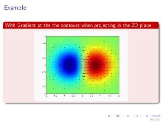
Because
M
y1=1
M
y2=1 · · · M
yN =1 applies only to δl,yi
N
j=1 p (yj|xj, Θg)
82 / 126](https://image.slidesharecdn.com/04-151212035340/85/07-Machine-Learning-Expectation-Maximization-195-320.jpg)
![Images/
Thus
We have that for
M
y1=1 · · · M
yN =1
N
i=1 log [αyi
pyi
(xi|θyi
)] N
j=1 p (yj|xj, Θg
) = ∗
∗ =
M
y1=1
M
y2=1
· · ·
M
yN =1
N
i=1
M
l=1
δl,yi
log [αlpl (xi|θl)]
N
j=1
p (yj|xj, Θg
)
=
N
i=1
M
l=1
log [αlpl (xi|θl)]
M
y1=1
M
y2=1
· · ·
M
yN =1
δl,yi
N
j=1
p (yj|xj, Θg
)
Because
M
y1=1
M
y2=1 · · · M
yN =1 applies only to δl,yi
N
j=1 p (yj|xj, Θg)
82 / 126](https://image.slidesharecdn.com/04-151212035340/85/07-Machine-Learning-Expectation-Maximization-196-320.jpg)
![Images/
Thus
We have that for
M
y1=1 · · · M
yN =1
N
i=1 log [αyi
pyi
(xi|θyi
)] N
j=1 p (yj|xj, Θg
) = ∗
∗ =
M
y1=1
M
y2=1
· · ·
M
yN =1
N
i=1
M
l=1
δl,yi
log [αlpl (xi|θl)]
N
j=1
p (yj|xj, Θg
)
=
N
i=1
M
l=1
log [αlpl (xi|θl)]
M
y1=1
M
y2=1
· · ·
M
yN =1
δl,yi
N
j=1
p (yj|xj, Θg
)
Because
M
y1=1
M
y2=1 · · · M
yN =1 applies only to δl,yi
N
j=1 p (yj|xj, Θg)
82 / 126](https://image.slidesharecdn.com/04-151212035340/85/07-Machine-Learning-Expectation-Maximization-197-320.jpg)


![Images/
Thus
We can write Q in the following way
Q (Θ, Θg
) =
N
i=1
M
l=1
log [αlpl (xi|θl)] p (l|xi, Θg
)
=
N
i=1
M
l=1
log (αl) p (l|xi, Θg
) + ...
N
i=1
M
l=1
log (pl (xi|θl)) p (l|xi, Θg
) (38)
88 / 126](https://image.slidesharecdn.com/04-151212035340/85/07-Machine-Learning-Expectation-Maximization-213-320.jpg)
![Images/
Thus
We can write Q in the following way
Q (Θ, Θg
) =
N
i=1
M
l=1
log [αlpl (xi|θl)] p (l|xi, Θg
)
=
N
i=1
M
l=1
log (αl) p (l|xi, Θg
) + ...
N
i=1
M
l=1
log (pl (xi|θl)) p (l|xi, Θg
) (38)
88 / 126](https://image.slidesharecdn.com/04-151212035340/85/07-Machine-Learning-Expectation-Maximization-214-320.jpg)
![Images/
Thus
We can write Q in the following way
Q (Θ, Θg
) =
N
i=1
M
l=1
log [αlpl (xi|θl)] p (l|xi, Θg
)
=
N
i=1
M
l=1
log (αl) p (l|xi, Θg
) + ...
N
i=1
M
l=1
log (pl (xi|θl)) p (l|xi, Θg
) (38)
88 / 126](https://image.slidesharecdn.com/04-151212035340/85/07-Machine-Learning-Expectation-Maximization-215-320.jpg)


![Images/
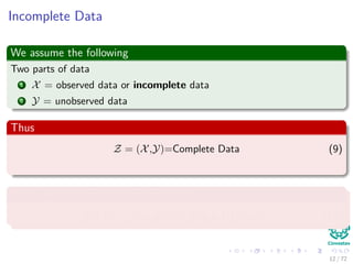
Thus, we have
Thus
If 2S − diag (S) = 0 =⇒ S = 0
Implying
1
2
N
i=1
p (l|xi, Θg
) [Σl − Nl,i] = 0 (58)
Or
Σl =
N
i=1 p (l|xi, Θg) Nl,i
N
i=1 p (l|xi, Θg)
=
N
i=1 p (l|xi, Θg) (xi − µl) (xi − µl)T
N
i=1 p (l|xi, Θg)
(59)
119 / 126](https://image.slidesharecdn.com/04-151212035340/85/07-Machine-Learning-Expectation-Maximization-284-320.jpg)
![Images/
Thus, we have
Thus
If 2S − diag (S) = 0 =⇒ S = 0
Implying
1
2
N
i=1
p (l|xi, Θg
) [Σl − Nl,i] = 0 (58)
Or
Σl =
N
i=1 p (l|xi, Θg) Nl,i
N
i=1 p (l|xi, Θg)
=
N
i=1 p (l|xi, Θg) (xi − µl) (xi − µl)T
N
i=1 p (l|xi, Θg)
(59)
119 / 126](https://image.slidesharecdn.com/04-151212035340/85/07-Machine-Learning-Expectation-Maximization-285-320.jpg)
![Images/
Thus, we have
Thus
If 2S − diag (S) = 0 =⇒ S = 0
Implying
1
2
N
i=1
p (l|xi, Θg
) [Σl − Nl,i] = 0 (58)
Or
Σl =
N
i=1 p (l|xi, Θg) Nl,i
N
i=1 p (l|xi, Θg)
=
N
i=1 p (l|xi, Θg) (xi − µl) (xi − µl)T
N
i=1 p (l|xi, Θg)
(59)
119 / 126](https://image.slidesharecdn.com/04-151212035340/85/07-Machine-Learning-Expectation-Maximization-286-320.jpg)


This document provides an introduction to the Expectation Maximization (EM) algorithm. EM is used to estimate parameters in statistical models when data is incomplete or has missing values. It is a two-step process: 1) Expectation step (E-step), where the expected value of the log likelihood is computed using the current estimate of parameters; 2) Maximization step (M-step), where the parameters are re-estimated to maximize the expected log likelihood found in the E-step. EM is commonly used for problems like clustering with mixture models and hidden Markov models. Applications of EM discussed include clustering data using mixture of Gaussian distributions, and training hidden Markov models for natural language processing tasks. The derivation of the EM algorithm and