Machine Learning for Data Mining
Important Issues
Andres Mendez-Vazquez
July 3, 2015
1 / 34
Images/cinvestav-
Outline
1 Bias-Variance Dilemma
Introduction
Measuring the difference between optimal and learned
The Bias-Variance
“Extreme” Example
2 Confusion Matrix
The Confusion Matrix
3 K-Cross Validation
Introduction
How to choose K
2 / 34
Images/cinvestav-
Outline
1 Bias-Variance Dilemma
Introduction
Measuring the difference between optimal and learned
The Bias-Variance
“Extreme” Example
2 Confusion Matrix
The Confusion Matrix
3 K-Cross Validation
Introduction
How to choose K
3 / 34
Images/cinvestav-
Introduction
What did we see until now?
The design of learning machines from two main points:
Statistical Point of View
Linear Algebra and Optimization Point of View
Going back to the probability models
We might think in the machine to be learned as a function g (x|D)....
Something as curve fitting...
Under a data set
D = {(xi, yi) |i = 1, 2, ..., N} (1)
Remark: Where the xi ∼ p (x|Θ)!!!
4 / 34
Images/cinvestav-
Thus, we have that
Two main functions
A function g (x|D) obtained using some algorithm!!!
E [y|x] the optimal regression...
Important
The key factor here is the dependence of the approximation on D.
Why?
The approximation may be very good for a specific training data set but
very bad for another.
This is the reason of studying fusion of information at decision level...
5 / 34
Images/cinvestav-
Outline
1 Bias-Variance Dilemma
Introduction
Measuring the difference between optimal and learned
The Bias-Variance
“Extreme” Example
2 Confusion Matrix
The Confusion Matrix
3 K-Cross Validation
Introduction
How to choose K
6 / 34
Images/cinvestav-
How do we measure the difference
We have that
Var(X) = E((X − µ)2
)
We can do that for our data
VarD (g (x|D)) = ED (g (x|D) − E [y|x])2
Now, if we add and subtract
ED [g (x|D)] (2)
Remark: The expected output of the machine g (x|D)
7 / 34
Images/cinvestav-
How do we measure the difference
We have that
Var(X) = E((X − µ)2
)
We can do that for our data
VarD (g (x|D)) = ED (g (x|D) − E [y|x])2
Now, if we add and subtract
ED [g (x|D)] (2)
Remark: The expected output of the machine g (x|D)
7 / 34
Images/cinvestav-
How do we measure the difference
We have that
Var(X) = E((X − µ)2
)
We can do that for our data
VarD (g (x|D)) = ED (g (x|D) − E [y|x])2
Now, if we add and subtract
ED [g (x|D)] (2)
Remark: The expected output of the machine g (x|D)
7 / 34
Images/cinvestav-
How do we measure the difference
We have that
Var(X) = E((X − µ)2
)
We can do that for our data
VarD (g (x|D)) = ED (g (x|D) − E [y|x])2
Now, if we add and subtract
ED [g (x|D)] (2)
Remark: The expected output of the machine g (x|D)
7 / 34
Images/cinvestav-
Thus, we have that
Or Original variance
VarD (g (x|D)) = ED (g (x|D) − E [y|x])2
= ED (g (x|D) − ED [g (x|D)] + ED [g (x|D)] − E [y|x])2
= ED (g (x|D) − ED [g (x|D)])2
+ ...
...2 ((g (x|D) − ED [g (x|D)])) (ED [g (x|D)] − E [y|x]) + ...
... (ED [g (x|D)] − E [y|x])2
Finally
ED (((g (x|D) − ED [g (x|D)])) (ED [g (x|D)] − E [y|x])) =? (3)
8 / 34
Images/cinvestav-
Outline
1 Bias-Variance Dilemma
Introduction
Measuring the difference between optimal and learned
The Bias-Variance
“Extreme” Example
2 Confusion Matrix
The Confusion Matrix
3 K-Cross Validation
Introduction
How to choose K
9 / 34
Images/cinvestav-
We have the Bias-Variance
Our Final Equation
ED (g (x|D) − E [y|x])2
= ED (g (x|D) − ED [g (x|D)])2
VARIANCE
+ (ED [g (x|D)] − E [y|x])2
BIAS
Where the variance
It represents the measure of the error between our machine g (x|D) and
the expected output of the machine under xi ∼ p (x|Θ).
Where the bias
It represents the quadratic error between the expected output of the
machine under xi ∼ p (x|Θ) and the expected output of the optimal
regression.
10 / 34
Images/cinvestav-
Remarks
We have then
Even if the estimator is unbiased, it can still result in a large mean square
error due to a large variance term.
The situation is more dire in a finite set of data D
We have then a trade-off:
1 Increasing the bias decreases the variance and vice versa.
2 This is known as the bias–variance dilemma.
11 / 34
Images/cinvestav-
Similar to...
Curve Fitting
If, for example, the adopted model is complex (many parameters involved)
with respect to the number N, the model will fit the idiosyncrasies of the
specific data set.
Thus
Thus, it will result in low bias but will yield high variance, as we change
from one data set to another data set.
Furthermore
If N grows we can have a more complex model to be fitted which reduces
bias and ensures low variance.
However, N is always finite!!!
12 / 34
Images/cinvestav-
Thus
You always need to compromise
However, you always have some a priori knowledge about the data
Allowing you to impose restrictions
Lowering the bias and the variance
Nevertheless
We have the following example to grasp better the bothersome
bias–variance dilemma.
13 / 34
Images/cinvestav-
Thus
You always need to compromise
However, you always have some a priori knowledge about the data
Allowing you to impose restrictions
Lowering the bias and the variance
Nevertheless
We have the following example to grasp better the bothersome
bias–variance dilemma.
13 / 34
Images/cinvestav-
Thus
You always need to compromise
However, you always have some a priori knowledge about the data
Allowing you to impose restrictions
Lowering the bias and the variance
Nevertheless
We have the following example to grasp better the bothersome
bias–variance dilemma.
13 / 34
Images/cinvestav-
For this
Assume
The data is generated by the following function
y =f (x) + ,
∼N 0, σ2
We know that
The optimum regressor is E [y|x] = f (x)
Furthermore
Assume that the randomness in the different training sets, D, is due to the
yi’s (Affected by noise), while the respective points, xi, are fixed.
14 / 34
Images/cinvestav-
Outline
1 Bias-Variance Dilemma
Introduction
Measuring the difference between optimal and learned
The Bias-Variance
“Extreme” Example
2 Confusion Matrix
The Confusion Matrix
3 K-Cross Validation
Introduction
How to choose K
15 / 34
Images/cinvestav-
Sampling the Space
Imagine that D ⊂ [x1, x2] in which x lies
For example, you can choose xi = x1 + x2−x1
N−1 (i − 1) with i = 1, 2, ..., N
16 / 34
Images/cinvestav-
Case 1
Choose the estimate of f (x), g (x|D), to be independent of D
For example, g (x) = w1x + w0
For example, the points are spread around (x, f (x))
17 / 34
Images/cinvestav-
Case 1
Choose the estimate of f (x), g (x|D), to be independent of D
For example, g (x) = w1x + w0
For example, the points are spread around (x, f (x))
0
Data Points
17 / 34
Images/cinvestav-
Case 1
Since g (x) is fixed
ED [g (x|D)] = g (x|D) ≡ g (x) (4)
With
VarD [g (x|D)] = 0 (5)
On the other hand
Because g (x) was chosen arbitrarily the expected bias must be large.
(ED [g (x|D)] − E [y|x])2
BIAS
(6)
18 / 34
Images/cinvestav-
Case 1
Since g (x) is fixed
ED [g (x|D)] = g (x|D) ≡ g (x) (4)
With
VarD [g (x|D)] = 0 (5)
On the other hand
Because g (x) was chosen arbitrarily the expected bias must be large.
(ED [g (x|D)] − E [y|x])2
BIAS
(6)
18 / 34
Images/cinvestav-
Case 1
Since g (x) is fixed
ED [g (x|D)] = g (x|D) ≡ g (x) (4)
With
VarD [g (x|D)] = 0 (5)
On the other hand
Because g (x) was chosen arbitrarily the expected bias must be large.
(ED [g (x|D)] − E [y|x])2
BIAS
(6)
18 / 34
Images/cinvestav-
Case 2
In the other hand
Now, g1 (x) corresponds to a polynomial of high degree so it can pass
through each training point in D.
Example of g1 (x)
19 / 34
Images/cinvestav-
Case 2
In the other hand
Now, g1 (x) corresponds to a polynomial of high degree so it can pass
through each training point in D.
Example of g1 (x)
0
Data Points
19 / 34
Images/cinvestav-
Case 2
Due to the zero mean of the noise source
ED [g1 (x|D)] = f (x) = E [y|x] for any x = xi (7)
Remark: At the training points the bias is zero.
However the variance increases
ED (g1 (x|D) − ED [g1 (x|D)])2
= ED (f (x) + − f (x))2
= σ2
, for x = xi, i = 1, 2, ..., N
In other words
The bias becomes zero (or approximately zero) but the variance is now
equal to the variance of the noise source.
20 / 34
Images/cinvestav-
Observations
First
Everything that has been said so far applies to both the regression and the
classification tasks.
However
Mean squared error is not the best way to measure the power of a classifier.
Think about
A classifier that send everything far away of the hyperplane!!! Away from
the values + − 1!!!
21 / 34
Images/cinvestav-
Outline
1 Bias-Variance Dilemma
Introduction
Measuring the difference between optimal and learned
The Bias-Variance
“Extreme” Example
2 Confusion Matrix
The Confusion Matrix
3 K-Cross Validation
Introduction
How to choose K
22 / 34
Images/cinvestav-
Introduction
Something Notable
In evaluating the performance of a classification system, the probability of
error is sometimes not the only quantity that assesses its performance
sufficiently.
For this assume a M-class classification task
An important issue is to know whether there are classes that exhibit a
higher tendency for confusion.
Where the confusion matrix
Confusion Matrix A = [Aij] is defined such that each element Aij is the
number of data points whose true class was i but where classified in class
j.
23 / 34
Images/cinvestav-
Thus
We have that
From A, one can directly extract the recall and precision values for each
class, along with the overall accuracy.
Recall - Ri
It is the percentage of data points with true class label i, which were
correctly classified in that class.
For example in a two-class problem
The recall of the first class is calculated as
R1 =
A11
A11 + A12
(8)
24 / 34
Images/cinvestav-
More
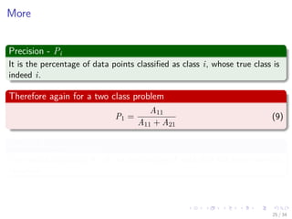
Precision - Pi
It is the percentage of data points classified as class i, whose true class is
indeed i.
Therefore again for a two class problem
P1 =
A11
A11 + A21
(9)
Overall Accuracy (Ac).
The overall accuracy, Ac, is the percentage of data that has been correctly
classified.
25 / 34
Images/cinvestav-
Thus, for a M-Class Problem
We have that
Ac =
1
N
M
i=1
Aii (10)
26 / 34
Images/cinvestav-
Outline
1 Bias-Variance Dilemma
Introduction
Measuring the difference between optimal and learned
The Bias-Variance
“Extreme” Example
2 Confusion Matrix
The Confusion Matrix
3 K-Cross Validation
Introduction
How to choose K
27 / 34
Images/cinvestav-
What we want
We want to measure
A quality measure to measure different classifiers (for different parameter
values).
We call that as
R(f ) = ED [L (y, f (x))] . (11)
Example: L (y, f (x)) = y − f (x) 2
2
More precisely
For different values γj of the parameter, we train a classifier f (x|γj) on
the training set.
28 / 34
Images/cinvestav-
Then, calculate the empirical Risk
Do you have any ideas?
Give me your best shot!!!
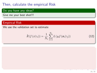
Empirical Risk
We use the validation set to estimate
ˆR (f (x|γi)) =
1
Nv
Nv
i=1
L (yif (xi|γj)) (12)
Thus, you follow the following procedure
1 Select the value γ∗ which achieves the smallest estimated error.
2 Re-train the classifier with parameter γ∗ on all data except the test
set (i.e. train + validation data).
3 Report error estimate ˆR (f (x|γi)) computed on the test set.
29 / 34
Images/cinvestav-
Idea
Something Notable
Each of the error estimates computed on validation set is computed from a
single example of a trained classifier. Can we improve the estimate?
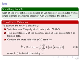
K-fold Cross Validation
To estimate the risk of a classifier f :
1 Split data into K equally sized parts (called "folds").
2 Train an instance fk of the classifier, using all folds except fold k as
training data.
3 Compute the cross validation (CV) estimate:
ˆRCV (f (x|γi)) =
1
Nv
Nv
i=1
L yif xk(i)|γj (13)
where k (i) is the fold containing xi.
30 / 34
Images/cinvestav-
Example
K = 5,k = 3
Train Train Validation Train Train
1 2 3 4 5
Actually, we have
Cross validation procedure does not involve the test data.
SPLIT THIS PART
Train Data + Validation Data Test
31 / 34
Images/cinvestav-
Example
K = 5,k = 3
Train Train Validation Train Train
1 2 3 4 5
Actually, we have
Cross validation procedure does not involve the test data.
SPLIT THIS PART
Train Data + Validation Data Test
31 / 34
Images/cinvestav-
Outline
1 Bias-Variance Dilemma
Introduction
Measuring the difference between optimal and learned
The Bias-Variance
“Extreme” Example
2 Confusion Matrix
The Confusion Matrix
3 K-Cross Validation
Introduction
How to choose K
32 / 34
Images/cinvestav-
How to choose K
Extremal cases
K = N, called leave one out cross validation (loocv)
K = 2
An often-cited problem with loocv is that we have to train many (= N)
classifiers, but there is also a deeper problem.
Argument 1: K should be small, e.g. K = 2
1 Unless we have a lot of data, variance between two distinct training
sets may be considerable.
2 Important concept: By removing substantial parts of the sample in
turn and at random, we can simulate this variance.
3 By removing a single point (loocv), we cannot make this variance
visible.
33 / 34
Images/cinvestav-
How to choose K
Argument 2: K should be large, e.g. K = N
1 Classifiers generally perform better when trained on larger data sets.
2 A small K means we substantially reduce the amount of training data
used to train each fk, so we may end up with weaker classifiers.
3 This way, we will systematically overestimate the risk.
Common recommendation: K = 5 to K = 10
Intuition:
1 K = 10 means number of samples removed from training is one order
of magnitude below training sample size.
2 This should not weaken the classifier considerably, but should be large
enough to make measure variance effects.
34 / 34

11 Machine Learning Important Issues in Machine Learning

  • 1.
    Machine Learning forData Mining Important Issues Andres Mendez-Vazquez July 3, 2015 1 / 34
  • 2.
    Images/cinvestav- Outline 1 Bias-Variance Dilemma Introduction Measuringthe difference between optimal and learned The Bias-Variance “Extreme” Example 2 Confusion Matrix The Confusion Matrix 3 K-Cross Validation Introduction How to choose K 2 / 34
  • 3.
    Images/cinvestav- Outline 1 Bias-Variance Dilemma Introduction Measuringthe difference between optimal and learned The Bias-Variance “Extreme” Example 2 Confusion Matrix The Confusion Matrix 3 K-Cross Validation Introduction How to choose K 3 / 34
  • 4.
    Images/cinvestav- Introduction What did wesee until now? The design of learning machines from two main points: Statistical Point of View Linear Algebra and Optimization Point of View Going back to the probability models We might think in the machine to be learned as a function g (x|D).... Something as curve fitting... Under a data set D = {(xi, yi) |i = 1, 2, ..., N} (1) Remark: Where the xi ∼ p (x|Θ)!!! 4 / 34
  • 5.
    Images/cinvestav- Introduction What did wesee until now? The design of learning machines from two main points: Statistical Point of View Linear Algebra and Optimization Point of View Going back to the probability models We might think in the machine to be learned as a function g (x|D).... Something as curve fitting... Under a data set D = {(xi, yi) |i = 1, 2, ..., N} (1) Remark: Where the xi ∼ p (x|Θ)!!! 4 / 34
  • 6.
    Images/cinvestav- Introduction What did wesee until now? The design of learning machines from two main points: Statistical Point of View Linear Algebra and Optimization Point of View Going back to the probability models We might think in the machine to be learned as a function g (x|D).... Something as curve fitting... Under a data set D = {(xi, yi) |i = 1, 2, ..., N} (1) Remark: Where the xi ∼ p (x|Θ)!!! 4 / 34
  • 7.
    Images/cinvestav- Introduction What did wesee until now? The design of learning machines from two main points: Statistical Point of View Linear Algebra and Optimization Point of View Going back to the probability models We might think in the machine to be learned as a function g (x|D).... Something as curve fitting... Under a data set D = {(xi, yi) |i = 1, 2, ..., N} (1) Remark: Where the xi ∼ p (x|Θ)!!! 4 / 34
  • 8.
    Images/cinvestav- Introduction What did wesee until now? The design of learning machines from two main points: Statistical Point of View Linear Algebra and Optimization Point of View Going back to the probability models We might think in the machine to be learned as a function g (x|D).... Something as curve fitting... Under a data set D = {(xi, yi) |i = 1, 2, ..., N} (1) Remark: Where the xi ∼ p (x|Θ)!!! 4 / 34
  • 9.
    Images/cinvestav- Introduction What did wesee until now? The design of learning machines from two main points: Statistical Point of View Linear Algebra and Optimization Point of View Going back to the probability models We might think in the machine to be learned as a function g (x|D).... Something as curve fitting... Under a data set D = {(xi, yi) |i = 1, 2, ..., N} (1) Remark: Where the xi ∼ p (x|Θ)!!! 4 / 34
  • 10.
    Images/cinvestav- Introduction What did wesee until now? The design of learning machines from two main points: Statistical Point of View Linear Algebra and Optimization Point of View Going back to the probability models We might think in the machine to be learned as a function g (x|D).... Something as curve fitting... Under a data set D = {(xi, yi) |i = 1, 2, ..., N} (1) Remark: Where the xi ∼ p (x|Θ)!!! 4 / 34
  • 11.
    Images/cinvestav- Thus, we havethat Two main functions A function g (x|D) obtained using some algorithm!!! E [y|x] the optimal regression... Important The key factor here is the dependence of the approximation on D. Why? The approximation may be very good for a specific training data set but very bad for another. This is the reason of studying fusion of information at decision level... 5 / 34
  • 12.
    Images/cinvestav- Thus, we havethat Two main functions A function g (x|D) obtained using some algorithm!!! E [y|x] the optimal regression... Important The key factor here is the dependence of the approximation on D. Why? The approximation may be very good for a specific training data set but very bad for another. This is the reason of studying fusion of information at decision level... 5 / 34
  • 13.
    Images/cinvestav- Thus, we havethat Two main functions A function g (x|D) obtained using some algorithm!!! E [y|x] the optimal regression... Important The key factor here is the dependence of the approximation on D. Why? The approximation may be very good for a specific training data set but very bad for another. This is the reason of studying fusion of information at decision level... 5 / 34
  • 14.
    Images/cinvestav- Thus, we havethat Two main functions A function g (x|D) obtained using some algorithm!!! E [y|x] the optimal regression... Important The key factor here is the dependence of the approximation on D. Why? The approximation may be very good for a specific training data set but very bad for another. This is the reason of studying fusion of information at decision level... 5 / 34
  • 15.
    Images/cinvestav- Thus, we havethat Two main functions A function g (x|D) obtained using some algorithm!!! E [y|x] the optimal regression... Important The key factor here is the dependence of the approximation on D. Why? The approximation may be very good for a specific training data set but very bad for another. This is the reason of studying fusion of information at decision level... 5 / 34
  • 16.
    Images/cinvestav- Outline 1 Bias-Variance Dilemma Introduction Measuringthe difference between optimal and learned The Bias-Variance “Extreme” Example 2 Confusion Matrix The Confusion Matrix 3 K-Cross Validation Introduction How to choose K 6 / 34
  • 17.
    Images/cinvestav- How do wemeasure the difference We have that Var(X) = E((X − µ)2 ) We can do that for our data VarD (g (x|D)) = ED (g (x|D) − E [y|x])2 Now, if we add and subtract ED [g (x|D)] (2) Remark: The expected output of the machine g (x|D) 7 / 34
  • 18.
    Images/cinvestav- How do wemeasure the difference We have that Var(X) = E((X − µ)2 ) We can do that for our data VarD (g (x|D)) = ED (g (x|D) − E [y|x])2 Now, if we add and subtract ED [g (x|D)] (2) Remark: The expected output of the machine g (x|D) 7 / 34
  • 19.
    Images/cinvestav- How do wemeasure the difference We have that Var(X) = E((X − µ)2 ) We can do that for our data VarD (g (x|D)) = ED (g (x|D) − E [y|x])2 Now, if we add and subtract ED [g (x|D)] (2) Remark: The expected output of the machine g (x|D) 7 / 34
  • 20.
    Images/cinvestav- How do wemeasure the difference We have that Var(X) = E((X − µ)2 ) We can do that for our data VarD (g (x|D)) = ED (g (x|D) − E [y|x])2 Now, if we add and subtract ED [g (x|D)] (2) Remark: The expected output of the machine g (x|D) 7 / 34
  • 21.
    Images/cinvestav- Thus, we havethat Or Original variance VarD (g (x|D)) = ED (g (x|D) − E [y|x])2 = ED (g (x|D) − ED [g (x|D)] + ED [g (x|D)] − E [y|x])2 = ED (g (x|D) − ED [g (x|D)])2 + ... ...2 ((g (x|D) − ED [g (x|D)])) (ED [g (x|D)] − E [y|x]) + ... ... (ED [g (x|D)] − E [y|x])2 Finally ED (((g (x|D) − ED [g (x|D)])) (ED [g (x|D)] − E [y|x])) =? (3) 8 / 34
  • 22.
    Images/cinvestav- Thus, we havethat Or Original variance VarD (g (x|D)) = ED (g (x|D) − E [y|x])2 = ED (g (x|D) − ED [g (x|D)] + ED [g (x|D)] − E [y|x])2 = ED (g (x|D) − ED [g (x|D)])2 + ... ...2 ((g (x|D) − ED [g (x|D)])) (ED [g (x|D)] − E [y|x]) + ... ... (ED [g (x|D)] − E [y|x])2 Finally ED (((g (x|D) − ED [g (x|D)])) (ED [g (x|D)] − E [y|x])) =? (3) 8 / 34
  • 23.
    Images/cinvestav- Thus, we havethat Or Original variance VarD (g (x|D)) = ED (g (x|D) − E [y|x])2 = ED (g (x|D) − ED [g (x|D)] + ED [g (x|D)] − E [y|x])2 = ED (g (x|D) − ED [g (x|D)])2 + ... ...2 ((g (x|D) − ED [g (x|D)])) (ED [g (x|D)] − E [y|x]) + ... ... (ED [g (x|D)] − E [y|x])2 Finally ED (((g (x|D) − ED [g (x|D)])) (ED [g (x|D)] − E [y|x])) =? (3) 8 / 34
  • 24.
    Images/cinvestav- Thus, we havethat Or Original variance VarD (g (x|D)) = ED (g (x|D) − E [y|x])2 = ED (g (x|D) − ED [g (x|D)] + ED [g (x|D)] − E [y|x])2 = ED (g (x|D) − ED [g (x|D)])2 + ... ...2 ((g (x|D) − ED [g (x|D)])) (ED [g (x|D)] − E [y|x]) + ... ... (ED [g (x|D)] − E [y|x])2 Finally ED (((g (x|D) − ED [g (x|D)])) (ED [g (x|D)] − E [y|x])) =? (3) 8 / 34
  • 25.
    Images/cinvestav- Outline 1 Bias-Variance Dilemma Introduction Measuringthe difference between optimal and learned The Bias-Variance “Extreme” Example 2 Confusion Matrix The Confusion Matrix 3 K-Cross Validation Introduction How to choose K 9 / 34
  • 26.
    Images/cinvestav- We have theBias-Variance Our Final Equation ED (g (x|D) − E [y|x])2 = ED (g (x|D) − ED [g (x|D)])2 VARIANCE + (ED [g (x|D)] − E [y|x])2 BIAS Where the variance It represents the measure of the error between our machine g (x|D) and the expected output of the machine under xi ∼ p (x|Θ). Where the bias It represents the quadratic error between the expected output of the machine under xi ∼ p (x|Θ) and the expected output of the optimal regression. 10 / 34
  • 27.
    Images/cinvestav- We have theBias-Variance Our Final Equation ED (g (x|D) − E [y|x])2 = ED (g (x|D) − ED [g (x|D)])2 VARIANCE + (ED [g (x|D)] − E [y|x])2 BIAS Where the variance It represents the measure of the error between our machine g (x|D) and the expected output of the machine under xi ∼ p (x|Θ). Where the bias It represents the quadratic error between the expected output of the machine under xi ∼ p (x|Θ) and the expected output of the optimal regression. 10 / 34
  • 28.
    Images/cinvestav- We have theBias-Variance Our Final Equation ED (g (x|D) − E [y|x])2 = ED (g (x|D) − ED [g (x|D)])2 VARIANCE + (ED [g (x|D)] − E [y|x])2 BIAS Where the variance It represents the measure of the error between our machine g (x|D) and the expected output of the machine under xi ∼ p (x|Θ). Where the bias It represents the quadratic error between the expected output of the machine under xi ∼ p (x|Θ) and the expected output of the optimal regression. 10 / 34
  • 29.
    Images/cinvestav- We have theBias-Variance Our Final Equation ED (g (x|D) − E [y|x])2 = ED (g (x|D) − ED [g (x|D)])2 VARIANCE + (ED [g (x|D)] − E [y|x])2 BIAS Where the variance It represents the measure of the error between our machine g (x|D) and the expected output of the machine under xi ∼ p (x|Θ). Where the bias It represents the quadratic error between the expected output of the machine under xi ∼ p (x|Θ) and the expected output of the optimal regression. 10 / 34
  • 30.
    Images/cinvestav- Remarks We have then Evenif the estimator is unbiased, it can still result in a large mean square error due to a large variance term. The situation is more dire in a finite set of data D We have then a trade-off: 1 Increasing the bias decreases the variance and vice versa. 2 This is known as the bias–variance dilemma. 11 / 34
  • 31.
    Images/cinvestav- Remarks We have then Evenif the estimator is unbiased, it can still result in a large mean square error due to a large variance term. The situation is more dire in a finite set of data D We have then a trade-off: 1 Increasing the bias decreases the variance and vice versa. 2 This is known as the bias–variance dilemma. 11 / 34
  • 32.
    Images/cinvestav- Remarks We have then Evenif the estimator is unbiased, it can still result in a large mean square error due to a large variance term. The situation is more dire in a finite set of data D We have then a trade-off: 1 Increasing the bias decreases the variance and vice versa. 2 This is known as the bias–variance dilemma. 11 / 34
  • 33.
    Images/cinvestav- Remarks We have then Evenif the estimator is unbiased, it can still result in a large mean square error due to a large variance term. The situation is more dire in a finite set of data D We have then a trade-off: 1 Increasing the bias decreases the variance and vice versa. 2 This is known as the bias–variance dilemma. 11 / 34
  • 34.
    Images/cinvestav- Similar to... Curve Fitting If,for example, the adopted model is complex (many parameters involved) with respect to the number N, the model will fit the idiosyncrasies of the specific data set. Thus Thus, it will result in low bias but will yield high variance, as we change from one data set to another data set. Furthermore If N grows we can have a more complex model to be fitted which reduces bias and ensures low variance. However, N is always finite!!! 12 / 34
  • 35.
    Images/cinvestav- Similar to... Curve Fitting If,for example, the adopted model is complex (many parameters involved) with respect to the number N, the model will fit the idiosyncrasies of the specific data set. Thus Thus, it will result in low bias but will yield high variance, as we change from one data set to another data set. Furthermore If N grows we can have a more complex model to be fitted which reduces bias and ensures low variance. However, N is always finite!!! 12 / 34
  • 36.
    Images/cinvestav- Similar to... Curve Fitting If,for example, the adopted model is complex (many parameters involved) with respect to the number N, the model will fit the idiosyncrasies of the specific data set. Thus Thus, it will result in low bias but will yield high variance, as we change from one data set to another data set. Furthermore If N grows we can have a more complex model to be fitted which reduces bias and ensures low variance. However, N is always finite!!! 12 / 34
  • 37.
    Images/cinvestav- Similar to... Curve Fitting If,for example, the adopted model is complex (many parameters involved) with respect to the number N, the model will fit the idiosyncrasies of the specific data set. Thus Thus, it will result in low bias but will yield high variance, as we change from one data set to another data set. Furthermore If N grows we can have a more complex model to be fitted which reduces bias and ensures low variance. However, N is always finite!!! 12 / 34
  • 38.
    Images/cinvestav- Thus You always needto compromise However, you always have some a priori knowledge about the data Allowing you to impose restrictions Lowering the bias and the variance Nevertheless We have the following example to grasp better the bothersome bias–variance dilemma. 13 / 34
  • 39.
    Images/cinvestav- Thus You always needto compromise However, you always have some a priori knowledge about the data Allowing you to impose restrictions Lowering the bias and the variance Nevertheless We have the following example to grasp better the bothersome bias–variance dilemma. 13 / 34
  • 40.
    Images/cinvestav- Thus You always needto compromise However, you always have some a priori knowledge about the data Allowing you to impose restrictions Lowering the bias and the variance Nevertheless We have the following example to grasp better the bothersome bias–variance dilemma. 13 / 34
  • 41.
    Images/cinvestav- For this Assume The datais generated by the following function y =f (x) + , ∼N 0, σ2 We know that The optimum regressor is E [y|x] = f (x) Furthermore Assume that the randomness in the different training sets, D, is due to the yi’s (Affected by noise), while the respective points, xi, are fixed. 14 / 34
  • 42.
    Images/cinvestav- For this Assume The datais generated by the following function y =f (x) + , ∼N 0, σ2 We know that The optimum regressor is E [y|x] = f (x) Furthermore Assume that the randomness in the different training sets, D, is due to the yi’s (Affected by noise), while the respective points, xi, are fixed. 14 / 34
  • 43.
    Images/cinvestav- For this Assume The datais generated by the following function y =f (x) + , ∼N 0, σ2 We know that The optimum regressor is E [y|x] = f (x) Furthermore Assume that the randomness in the different training sets, D, is due to the yi’s (Affected by noise), while the respective points, xi, are fixed. 14 / 34
  • 44.
    Images/cinvestav- Outline 1 Bias-Variance Dilemma Introduction Measuringthe difference between optimal and learned The Bias-Variance “Extreme” Example 2 Confusion Matrix The Confusion Matrix 3 K-Cross Validation Introduction How to choose K 15 / 34
  • 45.
    Images/cinvestav- Sampling the Space Imaginethat D ⊂ [x1, x2] in which x lies For example, you can choose xi = x1 + x2−x1 N−1 (i − 1) with i = 1, 2, ..., N 16 / 34
  • 46.
    Images/cinvestav- Case 1 Choose theestimate of f (x), g (x|D), to be independent of D For example, g (x) = w1x + w0 For example, the points are spread around (x, f (x)) 17 / 34
  • 47.
    Images/cinvestav- Case 1 Choose theestimate of f (x), g (x|D), to be independent of D For example, g (x) = w1x + w0 For example, the points are spread around (x, f (x)) 0 Data Points 17 / 34
  • 48.
    Images/cinvestav- Case 1 Since g(x) is fixed ED [g (x|D)] = g (x|D) ≡ g (x) (4) With VarD [g (x|D)] = 0 (5) On the other hand Because g (x) was chosen arbitrarily the expected bias must be large. (ED [g (x|D)] − E [y|x])2 BIAS (6) 18 / 34
  • 49.
    Images/cinvestav- Case 1 Since g(x) is fixed ED [g (x|D)] = g (x|D) ≡ g (x) (4) With VarD [g (x|D)] = 0 (5) On the other hand Because g (x) was chosen arbitrarily the expected bias must be large. (ED [g (x|D)] − E [y|x])2 BIAS (6) 18 / 34
  • 50.
    Images/cinvestav- Case 1 Since g(x) is fixed ED [g (x|D)] = g (x|D) ≡ g (x) (4) With VarD [g (x|D)] = 0 (5) On the other hand Because g (x) was chosen arbitrarily the expected bias must be large. (ED [g (x|D)] − E [y|x])2 BIAS (6) 18 / 34
  • 51.
    Images/cinvestav- Case 2 In theother hand Now, g1 (x) corresponds to a polynomial of high degree so it can pass through each training point in D. Example of g1 (x) 19 / 34
  • 52.
    Images/cinvestav- Case 2 In theother hand Now, g1 (x) corresponds to a polynomial of high degree so it can pass through each training point in D. Example of g1 (x) 0 Data Points 19 / 34
  • 53.
    Images/cinvestav- Case 2 Due tothe zero mean of the noise source ED [g1 (x|D)] = f (x) = E [y|x] for any x = xi (7) Remark: At the training points the bias is zero. However the variance increases ED (g1 (x|D) − ED [g1 (x|D)])2 = ED (f (x) + − f (x))2 = σ2 , for x = xi, i = 1, 2, ..., N In other words The bias becomes zero (or approximately zero) but the variance is now equal to the variance of the noise source. 20 / 34
  • 54.
    Images/cinvestav- Case 2 Due tothe zero mean of the noise source ED [g1 (x|D)] = f (x) = E [y|x] for any x = xi (7) Remark: At the training points the bias is zero. However the variance increases ED (g1 (x|D) − ED [g1 (x|D)])2 = ED (f (x) + − f (x))2 = σ2 , for x = xi, i = 1, 2, ..., N In other words The bias becomes zero (or approximately zero) but the variance is now equal to the variance of the noise source. 20 / 34
  • 55.
    Images/cinvestav- Case 2 Due tothe zero mean of the noise source ED [g1 (x|D)] = f (x) = E [y|x] for any x = xi (7) Remark: At the training points the bias is zero. However the variance increases ED (g1 (x|D) − ED [g1 (x|D)])2 = ED (f (x) + − f (x))2 = σ2 , for x = xi, i = 1, 2, ..., N In other words The bias becomes zero (or approximately zero) but the variance is now equal to the variance of the noise source. 20 / 34
  • 56.
    Images/cinvestav- Observations First Everything that hasbeen said so far applies to both the regression and the classification tasks. However Mean squared error is not the best way to measure the power of a classifier. Think about A classifier that send everything far away of the hyperplane!!! Away from the values + − 1!!! 21 / 34
  • 57.
    Images/cinvestav- Observations First Everything that hasbeen said so far applies to both the regression and the classification tasks. However Mean squared error is not the best way to measure the power of a classifier. Think about A classifier that send everything far away of the hyperplane!!! Away from the values + − 1!!! 21 / 34
  • 58.
    Images/cinvestav- Observations First Everything that hasbeen said so far applies to both the regression and the classification tasks. However Mean squared error is not the best way to measure the power of a classifier. Think about A classifier that send everything far away of the hyperplane!!! Away from the values + − 1!!! 21 / 34
  • 59.
    Images/cinvestav- Outline 1 Bias-Variance Dilemma Introduction Measuringthe difference between optimal and learned The Bias-Variance “Extreme” Example 2 Confusion Matrix The Confusion Matrix 3 K-Cross Validation Introduction How to choose K 22 / 34
  • 60.
    Images/cinvestav- Introduction Something Notable In evaluatingthe performance of a classification system, the probability of error is sometimes not the only quantity that assesses its performance sufficiently. For this assume a M-class classification task An important issue is to know whether there are classes that exhibit a higher tendency for confusion. Where the confusion matrix Confusion Matrix A = [Aij] is defined such that each element Aij is the number of data points whose true class was i but where classified in class j. 23 / 34
  • 61.
    Images/cinvestav- Introduction Something Notable In evaluatingthe performance of a classification system, the probability of error is sometimes not the only quantity that assesses its performance sufficiently. For this assume a M-class classification task An important issue is to know whether there are classes that exhibit a higher tendency for confusion. Where the confusion matrix Confusion Matrix A = [Aij] is defined such that each element Aij is the number of data points whose true class was i but where classified in class j. 23 / 34
  • 62.
    Images/cinvestav- Introduction Something Notable In evaluatingthe performance of a classification system, the probability of error is sometimes not the only quantity that assesses its performance sufficiently. For this assume a M-class classification task An important issue is to know whether there are classes that exhibit a higher tendency for confusion. Where the confusion matrix Confusion Matrix A = [Aij] is defined such that each element Aij is the number of data points whose true class was i but where classified in class j. 23 / 34
  • 63.
    Images/cinvestav- Thus We have that FromA, one can directly extract the recall and precision values for each class, along with the overall accuracy. Recall - Ri It is the percentage of data points with true class label i, which were correctly classified in that class. For example in a two-class problem The recall of the first class is calculated as R1 = A11 A11 + A12 (8) 24 / 34
  • 64.
    Images/cinvestav- Thus We have that FromA, one can directly extract the recall and precision values for each class, along with the overall accuracy. Recall - Ri It is the percentage of data points with true class label i, which were correctly classified in that class. For example in a two-class problem The recall of the first class is calculated as R1 = A11 A11 + A12 (8) 24 / 34
  • 65.
    Images/cinvestav- Thus We have that FromA, one can directly extract the recall and precision values for each class, along with the overall accuracy. Recall - Ri It is the percentage of data points with true class label i, which were correctly classified in that class. For example in a two-class problem The recall of the first class is calculated as R1 = A11 A11 + A12 (8) 24 / 34
  • 66.
    Images/cinvestav- More Precision - Pi Itis the percentage of data points classified as class i, whose true class is indeed i. Therefore again for a two class problem P1 = A11 A11 + A21 (9) Overall Accuracy (Ac). The overall accuracy, Ac, is the percentage of data that has been correctly classified. 25 / 34
  • 67.
    Images/cinvestav- More Precision - Pi Itis the percentage of data points classified as class i, whose true class is indeed i. Therefore again for a two class problem P1 = A11 A11 + A21 (9) Overall Accuracy (Ac). The overall accuracy, Ac, is the percentage of data that has been correctly classified. 25 / 34
  • 68.
    Images/cinvestav- More Precision - Pi Itis the percentage of data points classified as class i, whose true class is indeed i. Therefore again for a two class problem P1 = A11 A11 + A21 (9) Overall Accuracy (Ac). The overall accuracy, Ac, is the percentage of data that has been correctly classified. 25 / 34
  • 69.
    Images/cinvestav- Thus, for aM-Class Problem We have that Ac = 1 N M i=1 Aii (10) 26 / 34
  • 70.
    Images/cinvestav- Outline 1 Bias-Variance Dilemma Introduction Measuringthe difference between optimal and learned The Bias-Variance “Extreme” Example 2 Confusion Matrix The Confusion Matrix 3 K-Cross Validation Introduction How to choose K 27 / 34
  • 71.
    Images/cinvestav- What we want Wewant to measure A quality measure to measure different classifiers (for different parameter values). We call that as R(f ) = ED [L (y, f (x))] . (11) Example: L (y, f (x)) = y − f (x) 2 2 More precisely For different values γj of the parameter, we train a classifier f (x|γj) on the training set. 28 / 34
  • 72.
    Images/cinvestav- What we want Wewant to measure A quality measure to measure different classifiers (for different parameter values). We call that as R(f ) = ED [L (y, f (x))] . (11) Example: L (y, f (x)) = y − f (x) 2 2 More precisely For different values γj of the parameter, we train a classifier f (x|γj) on the training set. 28 / 34
  • 73.
    Images/cinvestav- What we want Wewant to measure A quality measure to measure different classifiers (for different parameter values). We call that as R(f ) = ED [L (y, f (x))] . (11) Example: L (y, f (x)) = y − f (x) 2 2 More precisely For different values γj of the parameter, we train a classifier f (x|γj) on the training set. 28 / 34
  • 74.
    Images/cinvestav- Then, calculate theempirical Risk Do you have any ideas? Give me your best shot!!! Empirical Risk We use the validation set to estimate ˆR (f (x|γi)) = 1 Nv Nv i=1 L (yif (xi|γj)) (12) Thus, you follow the following procedure 1 Select the value γ∗ which achieves the smallest estimated error. 2 Re-train the classifier with parameter γ∗ on all data except the test set (i.e. train + validation data). 3 Report error estimate ˆR (f (x|γi)) computed on the test set. 29 / 34
  • 75.
    Images/cinvestav- Then, calculate theempirical Risk Do you have any ideas? Give me your best shot!!! Empirical Risk We use the validation set to estimate ˆR (f (x|γi)) = 1 Nv Nv i=1 L (yif (xi|γj)) (12) Thus, you follow the following procedure 1 Select the value γ∗ which achieves the smallest estimated error. 2 Re-train the classifier with parameter γ∗ on all data except the test set (i.e. train + validation data). 3 Report error estimate ˆR (f (x|γi)) computed on the test set. 29 / 34
  • 76.
    Images/cinvestav- Then, calculate theempirical Risk Do you have any ideas? Give me your best shot!!! Empirical Risk We use the validation set to estimate ˆR (f (x|γi)) = 1 Nv Nv i=1 L (yif (xi|γj)) (12) Thus, you follow the following procedure 1 Select the value γ∗ which achieves the smallest estimated error. 2 Re-train the classifier with parameter γ∗ on all data except the test set (i.e. train + validation data). 3 Report error estimate ˆR (f (x|γi)) computed on the test set. 29 / 34
  • 77.
    Images/cinvestav- Then, calculate theempirical Risk Do you have any ideas? Give me your best shot!!! Empirical Risk We use the validation set to estimate ˆR (f (x|γi)) = 1 Nv Nv i=1 L (yif (xi|γj)) (12) Thus, you follow the following procedure 1 Select the value γ∗ which achieves the smallest estimated error. 2 Re-train the classifier with parameter γ∗ on all data except the test set (i.e. train + validation data). 3 Report error estimate ˆR (f (x|γi)) computed on the test set. 29 / 34
  • 78.
    Images/cinvestav- Then, calculate theempirical Risk Do you have any ideas? Give me your best shot!!! Empirical Risk We use the validation set to estimate ˆR (f (x|γi)) = 1 Nv Nv i=1 L (yif (xi|γj)) (12) Thus, you follow the following procedure 1 Select the value γ∗ which achieves the smallest estimated error. 2 Re-train the classifier with parameter γ∗ on all data except the test set (i.e. train + validation data). 3 Report error estimate ˆR (f (x|γi)) computed on the test set. 29 / 34
  • 79.
    Images/cinvestav- Idea Something Notable Each ofthe error estimates computed on validation set is computed from a single example of a trained classifier. Can we improve the estimate? K-fold Cross Validation To estimate the risk of a classifier f : 1 Split data into K equally sized parts (called "folds"). 2 Train an instance fk of the classifier, using all folds except fold k as training data. 3 Compute the cross validation (CV) estimate: ˆRCV (f (x|γi)) = 1 Nv Nv i=1 L yif xk(i)|γj (13) where k (i) is the fold containing xi. 30 / 34
  • 80.
    Images/cinvestav- Idea Something Notable Each ofthe error estimates computed on validation set is computed from a single example of a trained classifier. Can we improve the estimate? K-fold Cross Validation To estimate the risk of a classifier f : 1 Split data into K equally sized parts (called "folds"). 2 Train an instance fk of the classifier, using all folds except fold k as training data. 3 Compute the cross validation (CV) estimate: ˆRCV (f (x|γi)) = 1 Nv Nv i=1 L yif xk(i)|γj (13) where k (i) is the fold containing xi. 30 / 34
  • 81.
    Images/cinvestav- Idea Something Notable Each ofthe error estimates computed on validation set is computed from a single example of a trained classifier. Can we improve the estimate? K-fold Cross Validation To estimate the risk of a classifier f : 1 Split data into K equally sized parts (called "folds"). 2 Train an instance fk of the classifier, using all folds except fold k as training data. 3 Compute the cross validation (CV) estimate: ˆRCV (f (x|γi)) = 1 Nv Nv i=1 L yif xk(i)|γj (13) where k (i) is the fold containing xi. 30 / 34
  • 82.
    Images/cinvestav- Idea Something Notable Each ofthe error estimates computed on validation set is computed from a single example of a trained classifier. Can we improve the estimate? K-fold Cross Validation To estimate the risk of a classifier f : 1 Split data into K equally sized parts (called "folds"). 2 Train an instance fk of the classifier, using all folds except fold k as training data. 3 Compute the cross validation (CV) estimate: ˆRCV (f (x|γi)) = 1 Nv Nv i=1 L yif xk(i)|γj (13) where k (i) is the fold containing xi. 30 / 34
  • 83.
    Images/cinvestav- Idea Something Notable Each ofthe error estimates computed on validation set is computed from a single example of a trained classifier. Can we improve the estimate? K-fold Cross Validation To estimate the risk of a classifier f : 1 Split data into K equally sized parts (called "folds"). 2 Train an instance fk of the classifier, using all folds except fold k as training data. 3 Compute the cross validation (CV) estimate: ˆRCV (f (x|γi)) = 1 Nv Nv i=1 L yif xk(i)|γj (13) where k (i) is the fold containing xi. 30 / 34
  • 84.
    Images/cinvestav- Example K = 5,k= 3 Train Train Validation Train Train 1 2 3 4 5 Actually, we have Cross validation procedure does not involve the test data. SPLIT THIS PART Train Data + Validation Data Test 31 / 34
  • 85.
    Images/cinvestav- Example K = 5,k= 3 Train Train Validation Train Train 1 2 3 4 5 Actually, we have Cross validation procedure does not involve the test data. SPLIT THIS PART Train Data + Validation Data Test 31 / 34
  • 86.
    Images/cinvestav- Outline 1 Bias-Variance Dilemma Introduction Measuringthe difference between optimal and learned The Bias-Variance “Extreme” Example 2 Confusion Matrix The Confusion Matrix 3 K-Cross Validation Introduction How to choose K 32 / 34
  • 87.
    Images/cinvestav- How to chooseK Extremal cases K = N, called leave one out cross validation (loocv) K = 2 An often-cited problem with loocv is that we have to train many (= N) classifiers, but there is also a deeper problem. Argument 1: K should be small, e.g. K = 2 1 Unless we have a lot of data, variance between two distinct training sets may be considerable. 2 Important concept: By removing substantial parts of the sample in turn and at random, we can simulate this variance. 3 By removing a single point (loocv), we cannot make this variance visible. 33 / 34
  • 88.
    Images/cinvestav- How to chooseK Extremal cases K = N, called leave one out cross validation (loocv) K = 2 An often-cited problem with loocv is that we have to train many (= N) classifiers, but there is also a deeper problem. Argument 1: K should be small, e.g. K = 2 1 Unless we have a lot of data, variance between two distinct training sets may be considerable. 2 Important concept: By removing substantial parts of the sample in turn and at random, we can simulate this variance. 3 By removing a single point (loocv), we cannot make this variance visible. 33 / 34
  • 89.
    Images/cinvestav- How to chooseK Extremal cases K = N, called leave one out cross validation (loocv) K = 2 An often-cited problem with loocv is that we have to train many (= N) classifiers, but there is also a deeper problem. Argument 1: K should be small, e.g. K = 2 1 Unless we have a lot of data, variance between two distinct training sets may be considerable. 2 Important concept: By removing substantial parts of the sample in turn and at random, we can simulate this variance. 3 By removing a single point (loocv), we cannot make this variance visible. 33 / 34
  • 90.
    Images/cinvestav- How to chooseK Extremal cases K = N, called leave one out cross validation (loocv) K = 2 An often-cited problem with loocv is that we have to train many (= N) classifiers, but there is also a deeper problem. Argument 1: K should be small, e.g. K = 2 1 Unless we have a lot of data, variance between two distinct training sets may be considerable. 2 Important concept: By removing substantial parts of the sample in turn and at random, we can simulate this variance. 3 By removing a single point (loocv), we cannot make this variance visible. 33 / 34
  • 91.
    Images/cinvestav- How to chooseK Extremal cases K = N, called leave one out cross validation (loocv) K = 2 An often-cited problem with loocv is that we have to train many (= N) classifiers, but there is also a deeper problem. Argument 1: K should be small, e.g. K = 2 1 Unless we have a lot of data, variance between two distinct training sets may be considerable. 2 Important concept: By removing substantial parts of the sample in turn and at random, we can simulate this variance. 3 By removing a single point (loocv), we cannot make this variance visible. 33 / 34
  • 92.
    Images/cinvestav- How to chooseK Extremal cases K = N, called leave one out cross validation (loocv) K = 2 An often-cited problem with loocv is that we have to train many (= N) classifiers, but there is also a deeper problem. Argument 1: K should be small, e.g. K = 2 1 Unless we have a lot of data, variance between two distinct training sets may be considerable. 2 Important concept: By removing substantial parts of the sample in turn and at random, we can simulate this variance. 3 By removing a single point (loocv), we cannot make this variance visible. 33 / 34
  • 93.
    Images/cinvestav- How to chooseK Argument 2: K should be large, e.g. K = N 1 Classifiers generally perform better when trained on larger data sets. 2 A small K means we substantially reduce the amount of training data used to train each fk, so we may end up with weaker classifiers. 3 This way, we will systematically overestimate the risk. Common recommendation: K = 5 to K = 10 Intuition: 1 K = 10 means number of samples removed from training is one order of magnitude below training sample size. 2 This should not weaken the classifier considerably, but should be large enough to make measure variance effects. 34 / 34
  • 94.
    Images/cinvestav- How to chooseK Argument 2: K should be large, e.g. K = N 1 Classifiers generally perform better when trained on larger data sets. 2 A small K means we substantially reduce the amount of training data used to train each fk, so we may end up with weaker classifiers. 3 This way, we will systematically overestimate the risk. Common recommendation: K = 5 to K = 10 Intuition: 1 K = 10 means number of samples removed from training is one order of magnitude below training sample size. 2 This should not weaken the classifier considerably, but should be large enough to make measure variance effects. 34 / 34
  • 95.
    Images/cinvestav- How to chooseK Argument 2: K should be large, e.g. K = N 1 Classifiers generally perform better when trained on larger data sets. 2 A small K means we substantially reduce the amount of training data used to train each fk, so we may end up with weaker classifiers. 3 This way, we will systematically overestimate the risk. Common recommendation: K = 5 to K = 10 Intuition: 1 K = 10 means number of samples removed from training is one order of magnitude below training sample size. 2 This should not weaken the classifier considerably, but should be large enough to make measure variance effects. 34 / 34
  • 96.
    Images/cinvestav- How to chooseK Argument 2: K should be large, e.g. K = N 1 Classifiers generally perform better when trained on larger data sets. 2 A small K means we substantially reduce the amount of training data used to train each fk, so we may end up with weaker classifiers. 3 This way, we will systematically overestimate the risk. Common recommendation: K = 5 to K = 10 Intuition: 1 K = 10 means number of samples removed from training is one order of magnitude below training sample size. 2 This should not weaken the classifier considerably, but should be large enough to make measure variance effects. 34 / 34
  • 97.
    Images/cinvestav- How to chooseK Argument 2: K should be large, e.g. K = N 1 Classifiers generally perform better when trained on larger data sets. 2 A small K means we substantially reduce the amount of training data used to train each fk, so we may end up with weaker classifiers. 3 This way, we will systematically overestimate the risk. Common recommendation: K = 5 to K = 10 Intuition: 1 K = 10 means number of samples removed from training is one order of magnitude below training sample size. 2 This should not weaken the classifier considerably, but should be large enough to make measure variance effects. 34 / 34
  • 98.
    Images/cinvestav- How to chooseK Argument 2: K should be large, e.g. K = N 1 Classifiers generally perform better when trained on larger data sets. 2 A small K means we substantially reduce the amount of training data used to train each fk, so we may end up with weaker classifiers. 3 This way, we will systematically overestimate the risk. Common recommendation: K = 5 to K = 10 Intuition: 1 K = 10 means number of samples removed from training is one order of magnitude below training sample size. 2 This should not weaken the classifier considerably, but should be large enough to make measure variance effects. 34 / 34