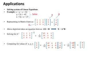
Basics of Matrix Algebra
Orated by:
Khushboo Gupta
AGENDA
• Definition and Nomenclature
• Matrix Equality
• Matrix Types
• Matrix Operations
• Independent vs. Dependent Vectors and Matrix Rank
• Matrix Determinant
• Matrix Inverse
• Examples
• Eigen values and vectors
• Applications
Definition and Nomenclature
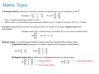
• Rectangular array of numbers arranged in rows and columns represented generally as A, B,
or C.
• Number of rows and columns that a matrix has is called its dimension or order
• Numbers that appear in the rows and columns are its elements.
• Symbolically depicted as:
𝐴 𝟏𝟏 𝐴 𝟏𝟐 𝐴 𝟏𝟑
𝐴 𝟐𝟏 𝐴 𝟐𝟐 𝐴 𝟐𝟑
𝐴 𝟑𝟏 𝐴 𝟑𝟐 𝐴 𝟑𝟑
• First subscript refers to row number,second to column number.
• Another approach for representation: A = [ Aij ] where i = 1, 2 and j = 1, 2, 3, 4 which means 2
rows and 4 columns.
Aij
Matrix Equality
• Two matrices are equal if:
- Each matrix has same number of rows and columns.
- Corresponding elements within each matrix are equal
• Example:
A=
111 𝑥
𝑦 444
B=
111 222
333 444
C=
𝑙 𝑚 𝑛
𝑜 𝑝 𝑞
𝑟 𝑠 𝑡
• Matrix C is not equal to A or B, because C has more columns than A or B.
Matrix Types
1) Transpose Matrix; wherein row becomes columns of original matrix, say A, denoted as A’ or A
T
Example: A=
1 3 4
2 5 7
A’ or AT=
1
3
2
5
4 7
• Row 1 of matrix A becomes column 1 of A';
• Matrix order is reversed after being transposed as Matrix A is 2 x 3 matrix, but matrix A' is a 3 x 2 matrix.
2) Vectors; wherein there exist only one column or one row, chiefly of two types: column vectors and
row vectors.
Example: matrix A is a column vector, and matrix A' is a row vector as shown below:
A=
2
3
4
A’= 2 3 4
3) Square matrix: n x n matrix (same number of rows as columns). Several kinds of square matrix.
(i) Symmetric matrix: Transpose of a matrix is equal to itself. Example as shown below:
A= A’=
1 2
2 3
B= B’=
5 6 7
6 3 2
7 2 1
(ii) Diagonal matrix: Matrix with zeros in off-diagonal elements as shown below:
A=
5 0 0
0 5 0
0 0 5
B=
3 2
0 9
Diagonal Matrix Non-Diagonal Matrix
Also a Scalar Matrix
special kind of diagonal matrix with equal-valued elements along the diagonal
One more example is: C=
1 0
0 1 This is also called as Identity Matrix I
Matrix Types
(iii) Triangular matrix; again is of two types, chiefly:
a) Upper Triangular; if all the entries below the main diagonal/ principle diagonal are zero.
Eg.: U =
1 3 6
0 1 4
0 0 1
𝑈 𝟏𝟏 ⋯ 𝑈 𝟏𝒏
⋮ ⋱ ⋮
0 ⋯ 𝑈 𝒏𝒏
b) Lower Triangular; all the entries above the main diagonal are zero.
Eg.: L=
1 0 0
2 1 0
3 5 1
𝐿 𝟏𝟏 ⋯ 0
⋮ ⋱ ⋮
𝐿 𝒏𝟏 ⋯ 𝐿 𝟏𝒏
Conclusively, triangular matrix is one that is either lower triangular or upper triangular.
Generalized Eqn
Generalized Eqn
Other Types of Matrices
Matrix Name Description
Idempotent Matrix A matrix wherein A2=A
Involutory Matrix A matrix s.t. A2=I
Nilpotent Matrix A square matrix is nilpotent if there exists a
positive integer ‘m’ such that Am=0
Orthogonal matrix Square matrix which satisfies the condition
AT = A-1
Conjugate Matrix or Hermitian Matrix ( 𝐴) Obtained by negating r imaginary parts of A
matrix. Eg: A=
1 + 𝑖 2
3 4 − 2𝑖
Then,
𝐴 =
1 − 𝑖 2
3 4 + 2𝑖
Transposed Conjugate Matrix ( 𝐴T) Transpose conjugate matrix
( 𝐴T) =
1 − 𝑖 3
2 4 + 2𝑖
Matrix Operations
1) Addition and Subtraction
• Two matrices can be added or subtracted if they have same order.
• Just add or subtract corresponding elements.
• Example, consider matrix A and matrix B as below:
A=
1 2 3
7 8 9 2x3 B=
5 6 7
3 4 5 2x3
Thus, A + B =
1 + 5 2 + 6 3 + 7
7 + 3 8 + 4 9 + 5
=
6 8 10
10 12 14
And, A – B =
1 − 5 2 − 6 3 − 7
7 − 3 8 − 4 9 − 5
=
−4 − 4 −4
4 4 4
2) Scalar Multiplication: Multiply every element in the matrix by scalar number,
producing a new matrix, called a scalar multiple.
Example: if x = 5, and matrix A= 2 4
6 5
Then, x A = 5A = 5
2 4
6 5
=
10 20
30 25
3) Matrix Multiplication: matrix product, say AB is defined only when number of columns in A
equals number of rows in B.
• A is i x j matrix, B is j x k matrix.
• Matrix product AB results in matrix, say C of order i x k
• Each element in C can be computed according to: Cik = Σj AijBjk
• Here, Cik = the element in row i and column k from matrix C
Aij = the element in row i and column j from matrix A
Bjk = the element in row j and column k from matrix B
Σj = summation sign, which indicates that the aijbjk terms should be summed over j.
Example: A=
0 1 2
3 4 5 2x3B=
6 7
8 9
10 11
3x2
Let AB = Cof order 2x2. Using formula Cik = Σj AijBjk, we get:
C11 = Σ A1jBj1 = 0*6 + 1*8 +2*10 = 0 + 8 + 20 = 28
C12 = Σ A1jBj2 = 0*7 + 1*9 +2*11 = 0 + 9 + 22 = 31
C21 = Σ A2jBj1 = 3*6 + 4*8 +5*10 = = 18 + 32 + 50 = 100
C22 = Σ A2jBj2 = 3*7 + 4*9 +5*11 = 21 + 36 +55 = 112
C=
28 31
100 112
Matrix Operations
Properties of Matrix Addition, Scalar and Matrix Multiplication
4) Vector Multiplication; namely of 2 types:
(i) Vector Inner Product(Dot Product/ Scalar Product)If a and b are vectors, each with same
number of elements then, inner product of a and b is s and a'b = b'a = s
• Here, a and b are column vectors, each having n elements,
a' is transpose of a, which makes a' a row vector,
b' is transpose of b, which makes b' a row vector, and
s is a scalar; that is, s is a real number (not a matrix).
• Example: a=
1
2
3
b=
4
5
6
(ii) Vector Outer Product If a and b are vectors and C is their outer product shown as: ab'= C
- Here, a is a column vector, having m elements,
b is a column vector, having n elements,
b' is the transpose of b, which makes b' a row vector, and
C is a rectangular m x n matrix
• Unlike the inner product, outer product of two vectors produces a rectangular matrix, not a scalar.
• Example: a=
𝑣
𝑤
b=
𝑥
𝑦
𝑧
Matrix Operations
a'b = 1*4 + 2*5 + 3*6 = 4 + 10 + 18 = 32
C= ab’=
𝑣 ∗ 𝑥 𝑣 ∗ 𝑦 𝑣 ∗ 𝑧
𝑤 ∗ 𝑥 𝑤 ∗ 𝑦 𝑤 ∗ 𝑧
• Crucial in many matrix algebra applications, such as finding inverse of a matrix and solving
simultaneous linear equations.
• Three kinds of elementary matrix operations.
- Interchange two rows (columns).
- Multiply each element in a row (column) by a non-zero number.
- Multiply a row (column) by non-zero number, add the result to another row (or column).
• Operations on rows (columns): elementary row operations (elementary column operations).
• Elementary Operation Notation; shown below:
Elementary Matrix Operations
Operation Description Notation
Row Operations
1. Interchange rows i and j Ri <-->Rj
2. Multiply row i by s, where s ≠ 0 sRi -->Ri
3. Add s times row i to row j sRi + Rj -->Rj
Column
Operations
1. Interchange columns i and j Ci <-->Cj
2. Multiply column i by s, where s ≠ 0 sCi --> Ci
3. Add s times column i to column j sCi + Cj -->Cj
Elementary Matrix Operations
This introduced the concept of: Row Echelon Form (REF) and Reduced Row Echelon Form (RREF)
• Row echelon form if:
- First non-zero element in each row, called the leading entry, is 1.
- Each leading entry is in a column to the right of the leading entry in the previous row.
- Rows with all zero elements, if any, are below rows having a non-zero element
Example: Aref =
1 2 3 4
0 0 1 3
0 0 0 1
Bref =
1 2
0 1
0 0
- Row operations used to convert A into Aref is called as Gaussian Elimination
• Reduced row echelon form if:
- Matrix satisfies conditions for a row echelon form.
- Leading entry in each row is the only non-zero entry in its column.
Example: Arref =
1 2 0 0
0 0 1 0
0 0 0 1
- Row operations used to convert A (Aref) into Arref is called as Gauss–Jordan elimination
An Example to solve RREF (REF) using Elementary Row Transformations
• Vector is dependent on other, if it is a linear combination of other vectors, i.e. equal to sum of scalar
multiples of other vectors
• Suppose a = 2b + 3c, as shown: a = 2
1
2
+ 3
3
4
a =
11
16
• Need is to find Rank of a matrix
• Defined as: (a) maximum number of linearly independent column vectors in matrix
(b) the maximum number of linearly independent row vectors in the matrix.
• For an r x c matrix,
- If r is less than c, then maximum rank of the matrix is r.
- If r is greater than c, then the maximum rank of the matrix is c.
• For Null matrix rank equals zero only.
To Find Rank
• Maximum number of linearly independent vectors in a matrix equals to number of non-zero rows in
its row echelon matrix.
• Now transform matrix into REF, count number of non-zero rows.
• Consider matrix A and its Aref as shown: A =
0 1 2
1 2 1
2 7 8
Aref=
1 2 1
0 1 2
0 0 0
• Since, Aref has two non-zero rows, i.e., two independent row vector, thus, A has rank equals 2
Independent vs. Dependent Vectors and Matrix Rank
Matrix Rank
Null Matrix
O =
0 0
0 0
Matrix Determinant
• Only of square matrix
• Notation: Det|A| or |A| |A|=
• Determinant Computation: A is a 2 x 2 matrix above, with elements Aij, then:






2221
1211
aa
aa
21122211 aaaaA 
Properties
1 |A|=|A'|.
2 If a row or column of A = 0, then |A|= 0.
3 If every value in a row or column is multiplied by k, then |A| = k|A|.
4 If two rows or columns are identical, |A| = 0.
5 |A| remains unchanged if each element of a row or each element
multiplied by a constant, is added to any other row.
6 |AB| = |A| |B|
7 Det of a diagonal matrix = product of the diagonal elements
Inverse of a Matrix (A-1)
• For an n  n matrix A, there may be a B such that AB = I = BA.
• Analogous to a reciprocal
• A matrix which has an inverse (no inverse) is nonsingular (singular).
• An inverse exists only if
Properties of inverse matrices
Computation
If and |A|  0
0A
  111 --
ABAB 

   '11 -
AA' 

  AA 
11-







dc
ba
A









ac
bd-
)det(
11
A
A
Generalized formula:
A-1 = 1
𝐷𝑒𝑡|𝑨| (adjoint(A))
Example to solve Inverse of matrix A
Given matrix A =
3 0 2
2 0 −2
0 1 1
Step 1: Calculate matrix Minor as shown below:
Step 2: Find Cofactor Matrix as shown
=
Step 3: Find Adjoint (Adjugate) of matrix by transposing the matrix obtained in step 2
as shown
Step 4: Find Determinant as
Step 5: Multiply the Adj by 1/Determinant as:
Example to solve Inverse of matrix A
Thus Det|A|= 3×2 - 0×2 + 2×2 = 10
Adjoint represented as ‘adj’
Eigen values and vectors
• Represented as A·v=λ·v, where, A is n-by-n matrix, v is a non-zero n-by-1
vector and λ is a scalar (which may be either real or complex).
• Any value of λ for which equation above has a solution is known as an
eigenvalue of A.
• Vector, v corresponding to this value is an eigenvector.
• Rewriting eigenvalue problem as:
• Above equation is called characteristic eqn with nth order polynomial in λ with
n roots called eigenvalues of A.
A·v-λ·v=0 or A·v-λ·I·v=0 or (A-λ·I)·v=0
If v is non-zero, this equation will only have a solution if |A-λ·I|=0
EXAMPLE
Characteristic Eqn
Eigen values
Eigen values and vectors Contd…
• For 2 eigen values λ1 and λ2 , there will be two eigen vectors, say v1 and v2, respectively.
• Solving further for λ1 as
Thus,
Similarly taking λ2, solve for v2 as
Applications
• Solving system of Linear Equations
• Example: x + y + z = 62
y + 5z = -42
x + 5y - z = 27
• Representing in Matrix Form as:
• Above depiction takes an equation form as: AX = B X = A-1B
• Solving for A-1
• Computing for values of x, y, z:
Solve
A
X B
REFERENCES
• Robbiano, Lorenzo. "Operations with Matrices." Linear algebra.
Springer Milan, 2011. 25-48.
• Marcus, Marvin. "Linear operations on matrices." The American
Mathematical Monthly 69.9 (1962): 837-847.
• Gantmakher, Feliks Ruvimovich. The theory of matrices. Vol. 131.
American Mathematical Soc., 1998.
• Leon, Steven J. Linear algebra with applications. New York:
Macmillan, 1980.
• Jang, Jyh-Shing Roger, Chuen-Tsai Sun, and Eiji Mizutani. "Neuro-
fuzzy and soft computing, a computational approach to learning and
machine intelligence." (1997).
THANK YOU

matrix algebra

  • 1.
    Basics of MatrixAlgebra Orated by: Khushboo Gupta
  • 2.
    AGENDA • Definition andNomenclature • Matrix Equality • Matrix Types • Matrix Operations • Independent vs. Dependent Vectors and Matrix Rank • Matrix Determinant • Matrix Inverse • Examples • Eigen values and vectors • Applications
  • 3.
    Definition and Nomenclature •Rectangular array of numbers arranged in rows and columns represented generally as A, B, or C. • Number of rows and columns that a matrix has is called its dimension or order • Numbers that appear in the rows and columns are its elements. • Symbolically depicted as: 𝐴 𝟏𝟏 𝐴 𝟏𝟐 𝐴 𝟏𝟑 𝐴 𝟐𝟏 𝐴 𝟐𝟐 𝐴 𝟐𝟑 𝐴 𝟑𝟏 𝐴 𝟑𝟐 𝐴 𝟑𝟑 • First subscript refers to row number,second to column number. • Another approach for representation: A = [ Aij ] where i = 1, 2 and j = 1, 2, 3, 4 which means 2 rows and 4 columns. Aij Matrix Equality • Two matrices are equal if: - Each matrix has same number of rows and columns. - Corresponding elements within each matrix are equal • Example: A= 111 𝑥 𝑦 444 B= 111 222 333 444 C= 𝑙 𝑚 𝑛 𝑜 𝑝 𝑞 𝑟 𝑠 𝑡 • Matrix C is not equal to A or B, because C has more columns than A or B.
  • 4.
    Matrix Types 1) TransposeMatrix; wherein row becomes columns of original matrix, say A, denoted as A’ or A T Example: A= 1 3 4 2 5 7 A’ or AT= 1 3 2 5 4 7 • Row 1 of matrix A becomes column 1 of A'; • Matrix order is reversed after being transposed as Matrix A is 2 x 3 matrix, but matrix A' is a 3 x 2 matrix. 2) Vectors; wherein there exist only one column or one row, chiefly of two types: column vectors and row vectors. Example: matrix A is a column vector, and matrix A' is a row vector as shown below: A= 2 3 4 A’= 2 3 4 3) Square matrix: n x n matrix (same number of rows as columns). Several kinds of square matrix. (i) Symmetric matrix: Transpose of a matrix is equal to itself. Example as shown below: A= A’= 1 2 2 3 B= B’= 5 6 7 6 3 2 7 2 1 (ii) Diagonal matrix: Matrix with zeros in off-diagonal elements as shown below: A= 5 0 0 0 5 0 0 0 5 B= 3 2 0 9 Diagonal Matrix Non-Diagonal Matrix Also a Scalar Matrix
  • 5.
    special kind ofdiagonal matrix with equal-valued elements along the diagonal One more example is: C= 1 0 0 1 This is also called as Identity Matrix I Matrix Types (iii) Triangular matrix; again is of two types, chiefly: a) Upper Triangular; if all the entries below the main diagonal/ principle diagonal are zero. Eg.: U = 1 3 6 0 1 4 0 0 1 𝑈 𝟏𝟏 ⋯ 𝑈 𝟏𝒏 ⋮ ⋱ ⋮ 0 ⋯ 𝑈 𝒏𝒏 b) Lower Triangular; all the entries above the main diagonal are zero. Eg.: L= 1 0 0 2 1 0 3 5 1 𝐿 𝟏𝟏 ⋯ 0 ⋮ ⋱ ⋮ 𝐿 𝒏𝟏 ⋯ 𝐿 𝟏𝒏 Conclusively, triangular matrix is one that is either lower triangular or upper triangular. Generalized Eqn Generalized Eqn
  • 6.
    Other Types ofMatrices Matrix Name Description Idempotent Matrix A matrix wherein A2=A Involutory Matrix A matrix s.t. A2=I Nilpotent Matrix A square matrix is nilpotent if there exists a positive integer ‘m’ such that Am=0 Orthogonal matrix Square matrix which satisfies the condition AT = A-1 Conjugate Matrix or Hermitian Matrix ( 𝐴) Obtained by negating r imaginary parts of A matrix. Eg: A= 1 + 𝑖 2 3 4 − 2𝑖 Then, 𝐴 = 1 − 𝑖 2 3 4 + 2𝑖 Transposed Conjugate Matrix ( 𝐴T) Transpose conjugate matrix ( 𝐴T) = 1 − 𝑖 3 2 4 + 2𝑖
  • 7.
    Matrix Operations 1) Additionand Subtraction • Two matrices can be added or subtracted if they have same order. • Just add or subtract corresponding elements. • Example, consider matrix A and matrix B as below: A= 1 2 3 7 8 9 2x3 B= 5 6 7 3 4 5 2x3 Thus, A + B = 1 + 5 2 + 6 3 + 7 7 + 3 8 + 4 9 + 5 = 6 8 10 10 12 14 And, A – B = 1 − 5 2 − 6 3 − 7 7 − 3 8 − 4 9 − 5 = −4 − 4 −4 4 4 4 2) Scalar Multiplication: Multiply every element in the matrix by scalar number, producing a new matrix, called a scalar multiple. Example: if x = 5, and matrix A= 2 4 6 5 Then, x A = 5A = 5 2 4 6 5 = 10 20 30 25
  • 8.
    3) Matrix Multiplication:matrix product, say AB is defined only when number of columns in A equals number of rows in B. • A is i x j matrix, B is j x k matrix. • Matrix product AB results in matrix, say C of order i x k • Each element in C can be computed according to: Cik = Σj AijBjk • Here, Cik = the element in row i and column k from matrix C Aij = the element in row i and column j from matrix A Bjk = the element in row j and column k from matrix B Σj = summation sign, which indicates that the aijbjk terms should be summed over j. Example: A= 0 1 2 3 4 5 2x3B= 6 7 8 9 10 11 3x2 Let AB = Cof order 2x2. Using formula Cik = Σj AijBjk, we get: C11 = Σ A1jBj1 = 0*6 + 1*8 +2*10 = 0 + 8 + 20 = 28 C12 = Σ A1jBj2 = 0*7 + 1*9 +2*11 = 0 + 9 + 22 = 31 C21 = Σ A2jBj1 = 3*6 + 4*8 +5*10 = = 18 + 32 + 50 = 100 C22 = Σ A2jBj2 = 3*7 + 4*9 +5*11 = 21 + 36 +55 = 112 C= 28 31 100 112 Matrix Operations
  • 9.
    Properties of MatrixAddition, Scalar and Matrix Multiplication
  • 10.
    4) Vector Multiplication;namely of 2 types: (i) Vector Inner Product(Dot Product/ Scalar Product)If a and b are vectors, each with same number of elements then, inner product of a and b is s and a'b = b'a = s • Here, a and b are column vectors, each having n elements, a' is transpose of a, which makes a' a row vector, b' is transpose of b, which makes b' a row vector, and s is a scalar; that is, s is a real number (not a matrix). • Example: a= 1 2 3 b= 4 5 6 (ii) Vector Outer Product If a and b are vectors and C is their outer product shown as: ab'= C - Here, a is a column vector, having m elements, b is a column vector, having n elements, b' is the transpose of b, which makes b' a row vector, and C is a rectangular m x n matrix • Unlike the inner product, outer product of two vectors produces a rectangular matrix, not a scalar. • Example: a= 𝑣 𝑤 b= 𝑥 𝑦 𝑧 Matrix Operations a'b = 1*4 + 2*5 + 3*6 = 4 + 10 + 18 = 32 C= ab’= 𝑣 ∗ 𝑥 𝑣 ∗ 𝑦 𝑣 ∗ 𝑧 𝑤 ∗ 𝑥 𝑤 ∗ 𝑦 𝑤 ∗ 𝑧
  • 11.
    • Crucial inmany matrix algebra applications, such as finding inverse of a matrix and solving simultaneous linear equations. • Three kinds of elementary matrix operations. - Interchange two rows (columns). - Multiply each element in a row (column) by a non-zero number. - Multiply a row (column) by non-zero number, add the result to another row (or column). • Operations on rows (columns): elementary row operations (elementary column operations). • Elementary Operation Notation; shown below: Elementary Matrix Operations Operation Description Notation Row Operations 1. Interchange rows i and j Ri <-->Rj 2. Multiply row i by s, where s ≠ 0 sRi -->Ri 3. Add s times row i to row j sRi + Rj -->Rj Column Operations 1. Interchange columns i and j Ci <-->Cj 2. Multiply column i by s, where s ≠ 0 sCi --> Ci 3. Add s times column i to column j sCi + Cj -->Cj
  • 12.
    Elementary Matrix Operations Thisintroduced the concept of: Row Echelon Form (REF) and Reduced Row Echelon Form (RREF) • Row echelon form if: - First non-zero element in each row, called the leading entry, is 1. - Each leading entry is in a column to the right of the leading entry in the previous row. - Rows with all zero elements, if any, are below rows having a non-zero element Example: Aref = 1 2 3 4 0 0 1 3 0 0 0 1 Bref = 1 2 0 1 0 0 - Row operations used to convert A into Aref is called as Gaussian Elimination • Reduced row echelon form if: - Matrix satisfies conditions for a row echelon form. - Leading entry in each row is the only non-zero entry in its column. Example: Arref = 1 2 0 0 0 0 1 0 0 0 0 1 - Row operations used to convert A (Aref) into Arref is called as Gauss–Jordan elimination
  • 13.
    An Example tosolve RREF (REF) using Elementary Row Transformations
  • 14.
    • Vector isdependent on other, if it is a linear combination of other vectors, i.e. equal to sum of scalar multiples of other vectors • Suppose a = 2b + 3c, as shown: a = 2 1 2 + 3 3 4 a = 11 16 • Need is to find Rank of a matrix • Defined as: (a) maximum number of linearly independent column vectors in matrix (b) the maximum number of linearly independent row vectors in the matrix. • For an r x c matrix, - If r is less than c, then maximum rank of the matrix is r. - If r is greater than c, then the maximum rank of the matrix is c. • For Null matrix rank equals zero only. To Find Rank • Maximum number of linearly independent vectors in a matrix equals to number of non-zero rows in its row echelon matrix. • Now transform matrix into REF, count number of non-zero rows. • Consider matrix A and its Aref as shown: A = 0 1 2 1 2 1 2 7 8 Aref= 1 2 1 0 1 2 0 0 0 • Since, Aref has two non-zero rows, i.e., two independent row vector, thus, A has rank equals 2 Independent vs. Dependent Vectors and Matrix Rank Matrix Rank Null Matrix O = 0 0 0 0
  • 15.
    Matrix Determinant • Onlyof square matrix • Notation: Det|A| or |A| |A|= • Determinant Computation: A is a 2 x 2 matrix above, with elements Aij, then:       2221 1211 aa aa 21122211 aaaaA  Properties 1 |A|=|A'|. 2 If a row or column of A = 0, then |A|= 0. 3 If every value in a row or column is multiplied by k, then |A| = k|A|. 4 If two rows or columns are identical, |A| = 0. 5 |A| remains unchanged if each element of a row or each element multiplied by a constant, is added to any other row. 6 |AB| = |A| |B| 7 Det of a diagonal matrix = product of the diagonal elements
  • 16.
    Inverse of aMatrix (A-1) • For an n  n matrix A, there may be a B such that AB = I = BA. • Analogous to a reciprocal • A matrix which has an inverse (no inverse) is nonsingular (singular). • An inverse exists only if Properties of inverse matrices Computation If and |A|  0 0A   111 -- ABAB      '11 - AA'     AA  11-        dc ba A          ac bd- )det( 11 A A Generalized formula: A-1 = 1 𝐷𝑒𝑡|𝑨| (adjoint(A))
  • 17.
    Example to solveInverse of matrix A Given matrix A = 3 0 2 2 0 −2 0 1 1 Step 1: Calculate matrix Minor as shown below: Step 2: Find Cofactor Matrix as shown =
  • 18.
    Step 3: FindAdjoint (Adjugate) of matrix by transposing the matrix obtained in step 2 as shown Step 4: Find Determinant as Step 5: Multiply the Adj by 1/Determinant as: Example to solve Inverse of matrix A Thus Det|A|= 3×2 - 0×2 + 2×2 = 10 Adjoint represented as ‘adj’
  • 19.
    Eigen values andvectors • Represented as A·v=λ·v, where, A is n-by-n matrix, v is a non-zero n-by-1 vector and λ is a scalar (which may be either real or complex). • Any value of λ for which equation above has a solution is known as an eigenvalue of A. • Vector, v corresponding to this value is an eigenvector. • Rewriting eigenvalue problem as: • Above equation is called characteristic eqn with nth order polynomial in λ with n roots called eigenvalues of A. A·v-λ·v=0 or A·v-λ·I·v=0 or (A-λ·I)·v=0 If v is non-zero, this equation will only have a solution if |A-λ·I|=0 EXAMPLE Characteristic Eqn Eigen values
  • 20.
    Eigen values andvectors Contd… • For 2 eigen values λ1 and λ2 , there will be two eigen vectors, say v1 and v2, respectively. • Solving further for λ1 as Thus, Similarly taking λ2, solve for v2 as
  • 21.
    Applications • Solving systemof Linear Equations • Example: x + y + z = 62 y + 5z = -42 x + 5y - z = 27 • Representing in Matrix Form as: • Above depiction takes an equation form as: AX = B X = A-1B • Solving for A-1 • Computing for values of x, y, z: Solve A X B
  • 22.
    REFERENCES • Robbiano, Lorenzo."Operations with Matrices." Linear algebra. Springer Milan, 2011. 25-48. • Marcus, Marvin. "Linear operations on matrices." The American Mathematical Monthly 69.9 (1962): 837-847. • Gantmakher, Feliks Ruvimovich. The theory of matrices. Vol. 131. American Mathematical Soc., 1998. • Leon, Steven J. Linear algebra with applications. New York: Macmillan, 1980. • Jang, Jyh-Shing Roger, Chuen-Tsai Sun, and Eiji Mizutani. "Neuro- fuzzy and soft computing, a computational approach to learning and machine intelligence." (1997).
  • 23.