Downloaded 20 times


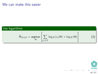
![Likelihood Principle
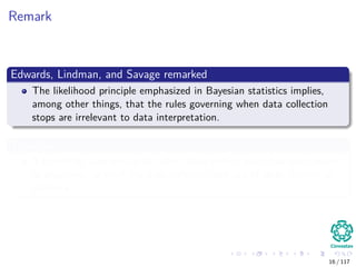
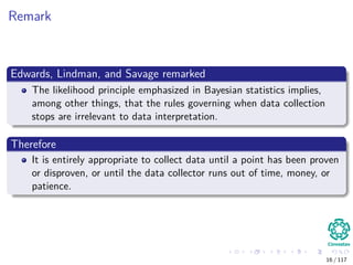
Remarks
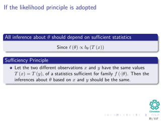
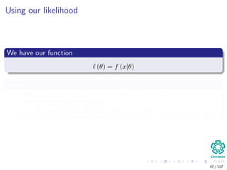
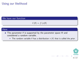
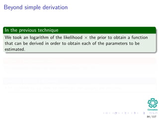
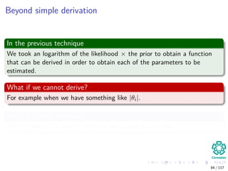
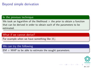
In the inference about θ, after x is observed, all relevant
experimental information is contained in the likelihood function
for the observed x.
There is an interesting example quoted by Lindley and Phillips in
1976 [1]
Originally by Leonard Savage
Leonard Savage
Leonard Jimmie Savage (born Leonard Ogashevitz; 20 November
1917 – 1 November 1971) was an American mathematician and
statistician.
Economist Milton Friedman said Savage was "one of the few people I
have met whom I would unhesitatingly call a genius.
6 / 117](https://image.slidesharecdn.com/2-200522084655/85/2-03-bayesian-estimation-9-320.jpg)
![Likelihood Principle
Remarks
In the inference about θ, after x is observed, all relevant
experimental information is contained in the likelihood function
for the observed x.
There is an interesting example quoted by Lindley and Phillips in
1976 [1]
Originally by Leonard Savage
Leonard Savage
Leonard Jimmie Savage (born Leonard Ogashevitz; 20 November
1917 – 1 November 1971) was an American mathematician and
statistician.
Economist Milton Friedman said Savage was "one of the few people I
have met whom I would unhesitatingly call a genius.
6 / 117](https://image.slidesharecdn.com/2-200522084655/85/2-03-bayesian-estimation-10-320.jpg)
![Likelihood Principle
Remarks
In the inference about θ, after x is observed, all relevant
experimental information is contained in the likelihood function
for the observed x.
There is an interesting example quoted by Lindley and Phillips in
1976 [1]
Originally by Leonard Savage
Leonard Savage
Leonard Jimmie Savage (born Leonard Ogashevitz; 20 November
1917 – 1 November 1971) was an American mathematician and
statistician.
Economist Milton Friedman said Savage was "one of the few people I
have met whom I would unhesitatingly call a genius.
6 / 117](https://image.slidesharecdn.com/2-200522084655/85/2-03-bayesian-estimation-11-320.jpg)


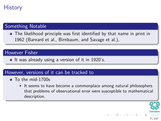


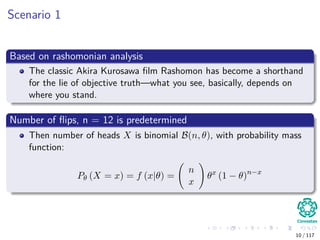
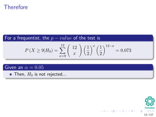
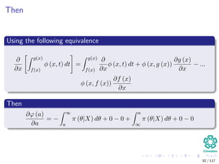
![Then if we use the following p − value analysis
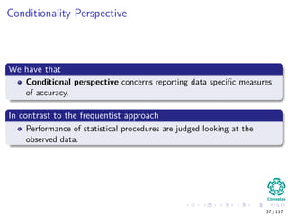
Definition [2, 3]
The p-value is defined as the probability, under the null hypothesis H0
about the unknown distribution F of the random variable X.
Very Unlike
Observation
Very Unlike
Observation
P-Value
More Likely Observation
Set of Possible Results
ProbabilityDensity
Observed
Data Point
12 / 117](https://image.slidesharecdn.com/2-200522084655/85/2-03-bayesian-estimation-23-320.jpg)

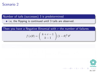
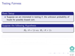
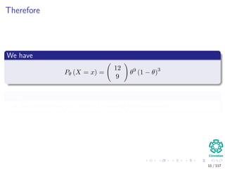
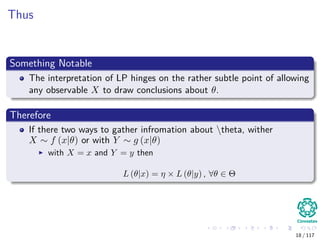
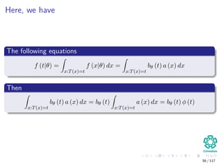
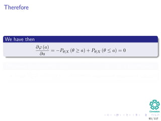
![Thus
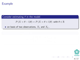
Likelihood Principle [4]
The Likelihood principle (LP) asserts that for inference on an
unknown quantity θ, all of the evidence from any observation X = x
with distribution X ∼ f (x|θ) lies in the likelihood function
L (θ|x) ∝ f (x|θ) , θ ∈ Θ
17 / 117](https://image.slidesharecdn.com/2-200522084655/85/2-03-bayesian-estimation-34-320.jpg)


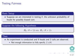
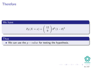
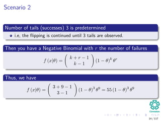
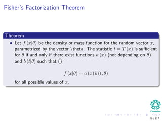
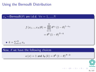
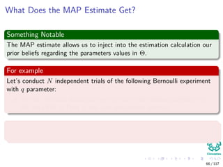
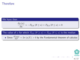
![The Basics
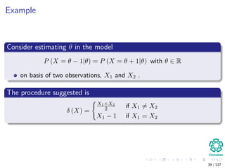
Sufficiency Principle
An statistic is sufficient with respect to a statistical model and its
associated unknown parameter if
"no other statistic that can be calculated from the same sample
provides any additional information as to the value of the parameter"[5]
However, as always
We want a definition to build upon it... as always
23 / 117](https://image.slidesharecdn.com/2-200522084655/85/2-03-bayesian-estimation-42-320.jpg)
![The Basics
Sufficiency Principle
An statistic is sufficient with respect to a statistical model and its
associated unknown parameter if
"no other statistic that can be calculated from the same sample
provides any additional information as to the value of the parameter"[5]
However, as always
We want a definition to build upon it... as always
23 / 117](https://image.slidesharecdn.com/2-200522084655/85/2-03-bayesian-estimation-43-320.jpg)
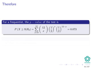
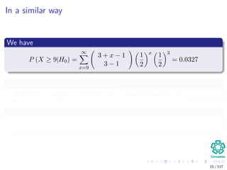
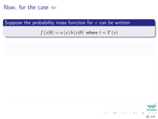
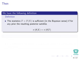
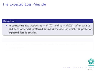
![A Basic Definition
Definition
A statistic t = T(X) is sufficient for underlying parameter θ precisely
if the conditional probability distribution of the data X, given the
statistic t = T(X), does not depend on the parameter θ [6].
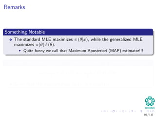
Something Notable
This agreement is non-philosophical, it is rather a consequence of
mathematics (measure theoretic considerations).
24 / 117](https://image.slidesharecdn.com/2-200522084655/85/2-03-bayesian-estimation-44-320.jpg)
![A Basic Definition
Definition
A statistic t = T(X) is sufficient for underlying parameter θ precisely
if the conditional probability distribution of the data X, given the
statistic t = T(X), does not depend on the parameter θ [6].
Something Notable
This agreement is non-philosophical, it is rather a consequence of
mathematics (measure theoretic considerations).
24 / 117](https://image.slidesharecdn.com/2-200522084655/85/2-03-bayesian-estimation-45-320.jpg)

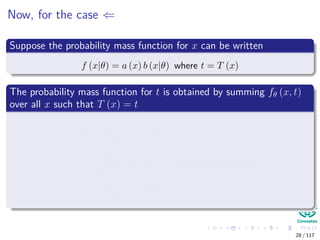
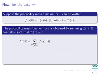
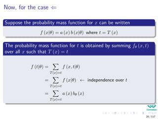
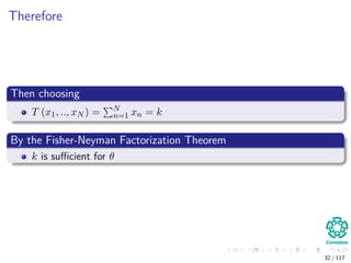
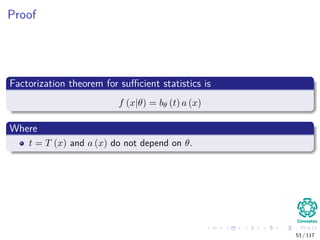
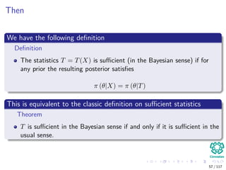
![Proof
First ⇒ (We will look only to the discrete case [7])
Suppose t = T (x) is sufficient for θ. Then, by definition
f (x|θ, T (x) = t) is independient of θ
Let f (x, t|θ) denote the joint density function or mass function for
(X, T (X))
Observe f (x|θ) = f (x, t|θ) then we have
f (x|θ) = f (x, t|θ)
= f (x|θ, t) f (t|θ) Bayesian
= a (x)
f (x|t)
b (t, θ)
f (t|θ)
Independence
27 / 117](https://image.slidesharecdn.com/2-200522084655/85/2-03-bayesian-estimation-48-320.jpg)
![Proof
First ⇒ (We will look only to the discrete case [7])
Suppose t = T (x) is sufficient for θ. Then, by definition
f (x|θ, T (x) = t) is independient of θ
Let f (x, t|θ) denote the joint density function or mass function for
(X, T (X))
Observe f (x|θ) = f (x, t|θ) then we have
f (x|θ) = f (x, t|θ)
= f (x|θ, t) f (t|θ) Bayesian
= a (x)
f (x|t)
b (t, θ)
f (t|θ)
Independence
27 / 117](https://image.slidesharecdn.com/2-200522084655/85/2-03-bayesian-estimation-49-320.jpg)
![Proof
First ⇒ (We will look only to the discrete case [7])
Suppose t = T (x) is sufficient for θ. Then, by definition
f (x|θ, T (x) = t) is independient of θ
Let f (x, t|θ) denote the joint density function or mass function for
(X, T (X))
Observe f (x|θ) = f (x, t|θ) then we have
f (x|θ) = f (x, t|θ)
= f (x|θ, t) f (t|θ) Bayesian
= a (x)
f (x|t)
b (t, θ)
f (t|θ)
Independence
27 / 117](https://image.slidesharecdn.com/2-200522084655/85/2-03-bayesian-estimation-50-320.jpg)
![Proof
First ⇒ (We will look only to the discrete case [7])
Suppose t = T (x) is sufficient for θ. Then, by definition
f (x|θ, T (x) = t) is independient of θ
Let f (x, t|θ) denote the joint density function or mass function for
(X, T (X))
Observe f (x|θ) = f (x, t|θ) then we have
f (x|θ) = f (x, t|θ)
= f (x|θ, t) f (t|θ) Bayesian
= a (x)
f (x|t)
b (t, θ)
f (t|θ)
Independence
27 / 117](https://image.slidesharecdn.com/2-200522084655/85/2-03-bayesian-estimation-51-320.jpg)
![Proof
First ⇒ (We will look only to the discrete case [7])
Suppose t = T (x) is sufficient for θ. Then, by definition
f (x|θ, T (x) = t) is independient of θ
Let f (x, t|θ) denote the joint density function or mass function for
(X, T (X))
Observe f (x|θ) = f (x, t|θ) then we have
f (x|θ) = f (x, t|θ)
= f (x|θ, t) f (t|θ) Bayesian
= a (x)
f (x|t)
b (t, θ)
f (t|θ)
Independence
27 / 117](https://image.slidesharecdn.com/2-200522084655/85/2-03-bayesian-estimation-52-320.jpg)
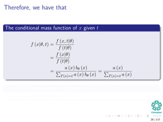


![The Lindley Paradox
Suppose y|θ ∼ N θ, 1
n
We wish to test H0 : θ = 0 vs the two sided alternative.
Suppose a Bayesian puts the prior P (θ = 0) = P (θ = 0) = 1
2
The 1
2 is uniformly spread over the interval [−M/2, M/2].
Suppose n = 40, 000 and y = 0.01 are observed
So,
√
ny = 2
44 / 117](https://image.slidesharecdn.com/2-200522084655/85/2-03-bayesian-estimation-78-320.jpg)
![The Lindley Paradox
Suppose y|θ ∼ N θ, 1
n
We wish to test H0 : θ = 0 vs the two sided alternative.
Suppose a Bayesian puts the prior P (θ = 0) = P (θ = 0) = 1
2
The 1
2 is uniformly spread over the interval [−M/2, M/2].
Suppose n = 40, 000 and y = 0.01 are observed
So,
√
ny = 2
44 / 117](https://image.slidesharecdn.com/2-200522084655/85/2-03-bayesian-estimation-79-320.jpg)
![The Lindley Paradox
Suppose y|θ ∼ N θ, 1
n
We wish to test H0 : θ = 0 vs the two sided alternative.
Suppose a Bayesian puts the prior P (θ = 0) = P (θ = 0) = 1
2
The 1
2 is uniformly spread over the interval [−M/2, M/2].
Suppose n = 40, 000 and y = 0.01 are observed
So,
√
ny = 2
44 / 117](https://image.slidesharecdn.com/2-200522084655/85/2-03-bayesian-estimation-80-320.jpg)


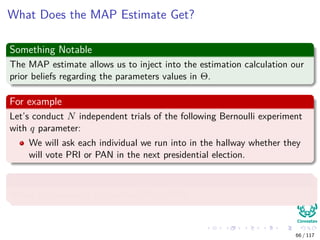

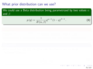
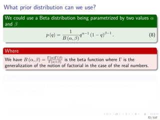
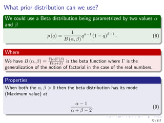
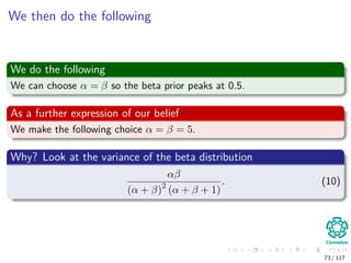
![Building the MAP estimate
Obviously we need a prior belief distribution
We have the following constraints:
The prior for q must be zero outside the [0, 1] interval.
Within the [0, 1] interval, we are free to specify our beliefs in any way
we wish.
In most cases, we would want to choose a distribution for the prior
beliefs that peaks somewhere in the [0, 1] interval.
We assume the following
The state of Colima has traditionally voted PRI in presidential
elections.
However, on account of the prevailing economic conditions, the voters
are more likely to vote PAN in the election in question.
71 / 117](https://image.slidesharecdn.com/2-200522084655/85/2-03-bayesian-estimation-138-320.jpg)
![Building the MAP estimate
Obviously we need a prior belief distribution
We have the following constraints:
The prior for q must be zero outside the [0, 1] interval.
Within the [0, 1] interval, we are free to specify our beliefs in any way
we wish.
In most cases, we would want to choose a distribution for the prior
beliefs that peaks somewhere in the [0, 1] interval.
We assume the following
The state of Colima has traditionally voted PRI in presidential
elections.
However, on account of the prevailing economic conditions, the voters
are more likely to vote PAN in the election in question.
71 / 117](https://image.slidesharecdn.com/2-200522084655/85/2-03-bayesian-estimation-139-320.jpg)
![Building the MAP estimate
Obviously we need a prior belief distribution
We have the following constraints:
The prior for q must be zero outside the [0, 1] interval.
Within the [0, 1] interval, we are free to specify our beliefs in any way
we wish.
In most cases, we would want to choose a distribution for the prior
beliefs that peaks somewhere in the [0, 1] interval.
We assume the following
The state of Colima has traditionally voted PRI in presidential
elections.
However, on account of the prevailing economic conditions, the voters
are more likely to vote PAN in the election in question.
71 / 117](https://image.slidesharecdn.com/2-200522084655/85/2-03-bayesian-estimation-140-320.jpg)
![Building the MAP estimate
Obviously we need a prior belief distribution
We have the following constraints:
The prior for q must be zero outside the [0, 1] interval.
Within the [0, 1] interval, we are free to specify our beliefs in any way
we wish.
In most cases, we would want to choose a distribution for the prior
beliefs that peaks somewhere in the [0, 1] interval.
We assume the following
The state of Colima has traditionally voted PRI in presidential
elections.
However, on account of the prevailing economic conditions, the voters
are more likely to vote PAN in the election in question.
71 / 117](https://image.slidesharecdn.com/2-200522084655/85/2-03-bayesian-estimation-141-320.jpg)
![Building the MAP estimate
Obviously we need a prior belief distribution
We have the following constraints:
The prior for q must be zero outside the [0, 1] interval.
Within the [0, 1] interval, we are free to specify our beliefs in any way
we wish.
In most cases, we would want to choose a distribution for the prior
beliefs that peaks somewhere in the [0, 1] interval.
We assume the following
The state of Colima has traditionally voted PRI in presidential
elections.
However, on account of the prevailing economic conditions, the voters
are more likely to vote PAN in the election in question.
71 / 117](https://image.slidesharecdn.com/2-200522084655/85/2-03-bayesian-estimation-142-320.jpg)
![Building the MAP estimate
Obviously we need a prior belief distribution
We have the following constraints:
The prior for q must be zero outside the [0, 1] interval.
Within the [0, 1] interval, we are free to specify our beliefs in any way
we wish.
In most cases, we would want to choose a distribution for the prior
beliefs that peaks somewhere in the [0, 1] interval.
We assume the following
The state of Colima has traditionally voted PRI in presidential
elections.
However, on account of the prevailing economic conditions, the voters
are more likely to vote PAN in the election in question.
71 / 117](https://image.slidesharecdn.com/2-200522084655/85/2-03-bayesian-estimation-143-320.jpg)
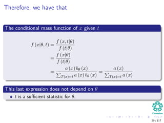
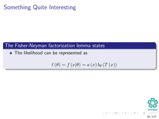
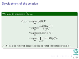
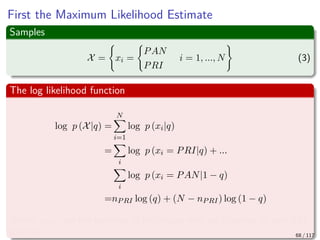
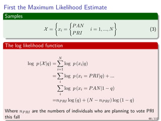
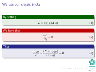
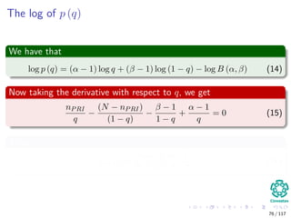
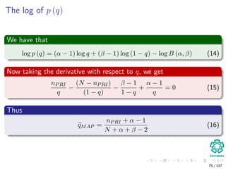
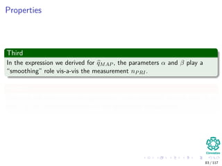
![Now, our MAP estimate for pMAP ...
We have then
pMAP = argmax
Θ
xi∈X
log p (xi|q) + log p (q)
(11)
Plugging back the ML
pMAP = argmax
Θ
[nPRI log q + (N − nPRI) log (1 − q) + log p (q)] (12)
Where
log p (q) = log
1
B (α, β)
qα−1
(1 − q)β−1
(13)
75 / 117](https://image.slidesharecdn.com/2-200522084655/85/2-03-bayesian-estimation-152-320.jpg)
![Now, our MAP estimate for pMAP ...
We have then
pMAP = argmax
Θ
xi∈X
log p (xi|q) + log p (q)
(11)
Plugging back the ML
pMAP = argmax
Θ
[nPRI log q + (N − nPRI) log (1 − q) + log p (q)] (12)
Where
log p (q) = log
1
B (α, β)
qα−1
(1 − q)β−1
(13)
75 / 117](https://image.slidesharecdn.com/2-200522084655/85/2-03-bayesian-estimation-153-320.jpg)
![Now, our MAP estimate for pMAP ...
We have then
pMAP = argmax
Θ
xi∈X
log p (xi|q) + log p (q)
(11)
Plugging back the ML
pMAP = argmax
Θ
[nPRI log q + (N − nPRI) log (1 − q) + log p (q)] (12)
Where
log p (q) = log
1
B (α, β)
qα−1
(1 − q)β−1
(13)
75 / 117](https://image.slidesharecdn.com/2-200522084655/85/2-03-bayesian-estimation-154-320.jpg)
![Another Example
Let X1, ..., Xn given θ are Poisson P (θ) with probability
f (xi|θ) = θxi
xi!
e−θ
Assume θ ∼ Γ (α, β) given by π (θ) ∝ θα−1e−βθ
The MAP is equal to
π (θ|X1, X2, ..., Xn) = π θ| Xi ∝ θ Xi+α−1
e−(n+β)θ
Basically Γ ( Xi + α − 1, n + β)
The mean is
E [θ|X] =
Xi + α
n + β
78 / 117](https://image.slidesharecdn.com/2-200522084655/85/2-03-bayesian-estimation-159-320.jpg)
![Another Example
Let X1, ..., Xn given θ are Poisson P (θ) with probability
f (xi|θ) = θxi
xi!
e−θ
Assume θ ∼ Γ (α, β) given by π (θ) ∝ θα−1e−βθ
The MAP is equal to
π (θ|X1, X2, ..., Xn) = π θ| Xi ∝ θ Xi+α−1
e−(n+β)θ
Basically Γ ( Xi + α − 1, n + β)
The mean is
E [θ|X] =
Xi + α
n + β
78 / 117](https://image.slidesharecdn.com/2-200522084655/85/2-03-bayesian-estimation-160-320.jpg)
![Another Example
Let X1, ..., Xn given θ are Poisson P (θ) with probability
f (xi|θ) = θxi
xi!
e−θ
Assume θ ∼ Γ (α, β) given by π (θ) ∝ θα−1e−βθ
The MAP is equal to
π (θ|X1, X2, ..., Xn) = π θ| Xi ∝ θ Xi+α−1
e−(n+β)θ
Basically Γ ( Xi + α − 1, n + β)
The mean is
E [θ|X] =
Xi + α
n + β
78 / 117](https://image.slidesharecdn.com/2-200522084655/85/2-03-bayesian-estimation-161-320.jpg)
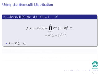
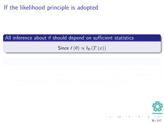
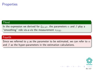
![Now, given the mean of the Γ
We can rewrite the mean as
E [θ|X] =
n
n + β
×
Xi
n
+
β
β + n
×
α
β
Given that the means are
Mean of MLE
Xi
n
Mean of the prior α
β
79 / 117](https://image.slidesharecdn.com/2-200522084655/85/2-03-bayesian-estimation-162-320.jpg)
![Now, given the mean of the Γ
We can rewrite the mean as
E [θ|X] =
n
n + β
×
Xi
n
+
β
β + n
×
α
β
Given that the means are
Mean of MLE
Xi
n
Mean of the prior α
β
79 / 117](https://image.slidesharecdn.com/2-200522084655/85/2-03-bayesian-estimation-163-320.jpg)


![Examples
Squared Error Loss
L (θ, a) = (θ − a)2
Absolute Loss
L (θ, a) = |θ − a|
0-1 Loss example
L (θ, a) = I [|θ − a| > m]
89 / 117](https://image.slidesharecdn.com/2-200522084655/85/2-03-bayesian-estimation-181-320.jpg)
![Examples
Squared Error Loss
L (θ, a) = (θ − a)2
Absolute Loss
L (θ, a) = |θ − a|
0-1 Loss example
L (θ, a) = I [|θ − a| > m]
89 / 117](https://image.slidesharecdn.com/2-200522084655/85/2-03-bayesian-estimation-182-320.jpg)
![Examples
Squared Error Loss
L (θ, a) = (θ − a)2
Absolute Loss
L (θ, a) = |θ − a|
0-1 Loss example
L (θ, a) = I [|θ − a| > m]
89 / 117](https://image.slidesharecdn.com/2-200522084655/85/2-03-bayesian-estimation-183-320.jpg)
![Clearly the easiest mathematically SEL
Additionally, it is linked with
EX|θ [θ − δ (X)]2
= V ar (δ (X)) + [bias (δ (X))]2
Where bias (δ (X)) = EX|θ [δ (X)] − θ
90 / 117](https://image.slidesharecdn.com/2-200522084655/85/2-03-bayesian-estimation-184-320.jpg)
![In another example
The median, m, of random variable X is defined as
P (X ≥ m) ≥
1
2
,
P (X ≤ m) ≤
1
2
Assuming the absolute loss
ϕ (a) =Eθ|X [|θ − a|]
=
θ≥a
(θ − a) π (θ|X) dθ +
θ≤a
(a − θ) π (θ|X) dθ
=
∞
a
(θ − a) π (θ|X) dθ +
a
∞
(a − θ) π (θ|X) dθ
91 / 117](https://image.slidesharecdn.com/2-200522084655/85/2-03-bayesian-estimation-185-320.jpg)
![In another example
The median, m, of random variable X is defined as
P (X ≥ m) ≥
1
2
,
P (X ≤ m) ≤
1
2
Assuming the absolute loss
ϕ (a) =Eθ|X [|θ − a|]
=
θ≥a
(θ − a) π (θ|X) dθ +
θ≤a
(a − θ) π (θ|X) dθ
=
∞
a
(θ − a) π (θ|X) dθ +
a
∞
(a − θ) π (θ|X) dθ
91 / 117](https://image.slidesharecdn.com/2-200522084655/85/2-03-bayesian-estimation-186-320.jpg)
![In another example
The median, m, of random variable X is defined as
P (X ≥ m) ≥
1
2
,
P (X ≤ m) ≤
1
2
Assuming the absolute loss
ϕ (a) =Eθ|X [|θ − a|]
=
θ≥a
(θ − a) π (θ|X) dθ +
θ≤a
(a − θ) π (θ|X) dθ
=
∞
a
(θ − a) π (θ|X) dθ +
a
∞
(a − θ) π (θ|X) dθ
91 / 117](https://image.slidesharecdn.com/2-200522084655/85/2-03-bayesian-estimation-187-320.jpg)
![In another example
The median, m, of random variable X is defined as
P (X ≥ m) ≥
1
2
,
P (X ≤ m) ≤
1
2
Assuming the absolute loss
ϕ (a) =Eθ|X [|θ − a|]
=
θ≥a
(θ − a) π (θ|X) dθ +
θ≤a
(a − θ) π (θ|X) dθ
=
∞
a
(θ − a) π (θ|X) dθ +
a
∞
(a − θ) π (θ|X) dθ
91 / 117](https://image.slidesharecdn.com/2-200522084655/85/2-03-bayesian-estimation-188-320.jpg)


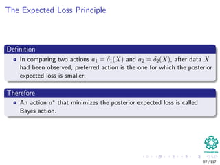
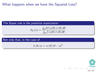
![Bayesian Expected Loss
Definition
Bayesian expected loss is the expectation of the loss function with
respect to posterior measure,
ρ (a, π) = Eθ|X [L (a, θ)] =
Θ
L (θ, a) π (θ|x) dθ
Here, we have an important principle
Referring to the less possible loss!!!
96 / 117](https://image.slidesharecdn.com/2-200522084655/85/2-03-bayesian-estimation-195-320.jpg)
![Bayesian Expected Loss
Definition
Bayesian expected loss is the expectation of the loss function with
respect to posterior measure,
ρ (a, π) = Eθ|X [L (a, θ)] =
Θ
L (θ, a) π (θ|x) dθ
Here, we have an important principle
Referring to the less possible loss!!!
96 / 117](https://image.slidesharecdn.com/2-200522084655/85/2-03-bayesian-estimation-196-320.jpg)

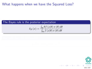
![Example
If the loss is squared error
The Bayes action a∗ is found by minimizing
ϕ (a) = Eθ|X (θ − a)2
= a2
− 2Eθ|X [θ] a + Eθ|Xθ2
Then, we want ϕ (a) = 0
Solving for it, we have a = Eθ|X [θ]
Additionally
ϕ (a) < 0 then a∗ = Eθ|X [θ] is a Bayesian Action.
99 / 117](https://image.slidesharecdn.com/2-200522084655/85/2-03-bayesian-estimation-200-320.jpg)
![Example
If the loss is squared error
The Bayes action a∗ is found by minimizing
ϕ (a) = Eθ|X (θ − a)2
= a2
− 2Eθ|X [θ] a + Eθ|Xθ2
Then, we want ϕ (a) = 0
Solving for it, we have a = Eθ|X [θ]
Additionally
ϕ (a) < 0 then a∗ = Eθ|X [θ] is a Bayesian Action.
99 / 117](https://image.slidesharecdn.com/2-200522084655/85/2-03-bayesian-estimation-201-320.jpg)
![Example
If the loss is squared error
The Bayes action a∗ is found by minimizing
ϕ (a) = Eθ|X (θ − a)2
= a2
− 2Eθ|X [θ] a + Eθ|Xθ2
Then, we want ϕ (a) = 0
Solving for it, we have a = Eθ|X [θ]
Additionally
ϕ (a) < 0 then a∗ = Eθ|X [θ] is a Bayesian Action.
99 / 117](https://image.slidesharecdn.com/2-200522084655/85/2-03-bayesian-estimation-202-320.jpg)

![A be the class of all possible realizations of δ(x), i.e.
actions
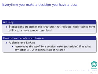
The Loss function L (θ, a) maps Θ × A −→ R
Defining a cost to the statistician when he takes the action a and the
true value of the parameter is θ.
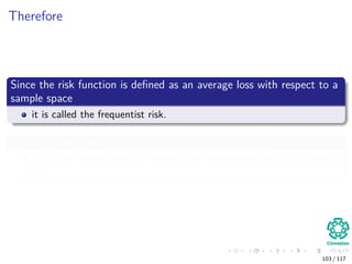
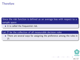
Then we can define a decision function called Risk
R (θ, δ) = EX|θ [L (θ|δ (X))] =
X
L (θ|δ (X)) f (x|θ) dx
A frequentist risk on the performance of δ.
102 / 117](https://image.slidesharecdn.com/2-200522084655/85/2-03-bayesian-estimation-206-320.jpg)
![A be the class of all possible realizations of δ(x), i.e.
actions
The Loss function L (θ, a) maps Θ × A −→ R
Defining a cost to the statistician when he takes the action a and the
true value of the parameter is θ.
Then we can define a decision function called Risk
R (θ, δ) = EX|θ [L (θ|δ (X))] =
X
L (θ|δ (X)) f (x|θ) dx
A frequentist risk on the performance of δ.
102 / 117](https://image.slidesharecdn.com/2-200522084655/85/2-03-bayesian-estimation-207-320.jpg)


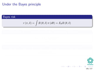
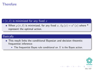
![Bayes Envelope Function Definition
Definition
The Bayes Envelope is the maximal reward rate a player could achieve
had he known in advance the relative frequencies of the other players.
In particular, we define the following function as
r (π, δ) = Eθ EX|θ [L (θ, δ (X))]
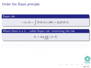
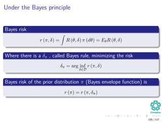
Therefore the Bayes action as Bayes Rules looks like
δ∗
(x) = arg min
δ∈D
r (π, δ)
106 / 117](https://image.slidesharecdn.com/2-200522084655/85/2-03-bayesian-estimation-218-320.jpg)
![Bayes Envelope Function Definition
Definition
The Bayes Envelope is the maximal reward rate a player could achieve
had he known in advance the relative frequencies of the other players.
In particular, we define the following function as
r (π, δ) = Eθ EX|θ [L (θ, δ (X))]
Therefore the Bayes action as Bayes Rules looks like
δ∗
(x) = arg min
δ∈D
r (π, δ)
106 / 117](https://image.slidesharecdn.com/2-200522084655/85/2-03-bayesian-estimation-219-320.jpg)
![Bayes Envelope Function Definition
Definition
The Bayes Envelope is the maximal reward rate a player could achieve
had he known in advance the relative frequencies of the other players.
In particular, we define the following function as
r (π, δ) = Eθ EX|θ [L (θ, δ (X))]
Therefore the Bayes action as Bayes Rules looks like
δ∗
(x) = arg min
δ∈D
r (π, δ)
106 / 117](https://image.slidesharecdn.com/2-200522084655/85/2-03-bayesian-estimation-220-320.jpg)

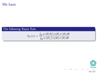
![Implications with the Expected Value
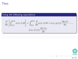
We have by the Fubini’s Theorem
r (π, δ) = Eθ EX|θ [L (θ, δ (X))]
= EX Eθ|X [L (θ, δ (X))]
Where the posterior expected loss
ρ (π, δ) = Eθ|X [L (θ, δ (X))]
110 / 117](https://image.slidesharecdn.com/2-200522084655/85/2-03-bayesian-estimation-225-320.jpg)
![Implications with the Expected Value
We have by the Fubini’s Theorem
r (π, δ) = Eθ EX|θ [L (θ, δ (X))]
= EX Eθ|X [L (θ, δ (X))]
Where the posterior expected loss
ρ (π, δ) = Eθ|X [L (θ, δ (X))]
110 / 117](https://image.slidesharecdn.com/2-200522084655/85/2-03-bayesian-estimation-226-320.jpg)


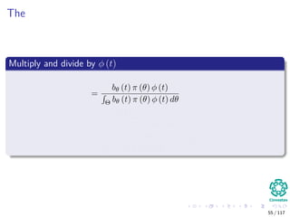
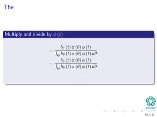
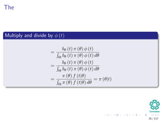
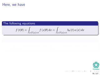
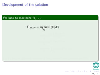
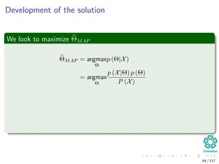
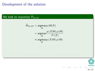
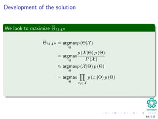
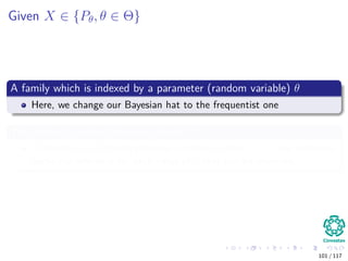
This document outlines an introduction to Bayesian estimation. It discusses key concepts like the likelihood principle, sufficiency, and Bayesian inference. The likelihood principle states that all experimental information about an unknown parameter is contained within the likelihood function. An example is provided testing the fairness of a coin using different data collection scenarios to illustrate how the likelihood function remains the same. The document also discusses the history of the likelihood principle and provides an outline of topics to be covered.