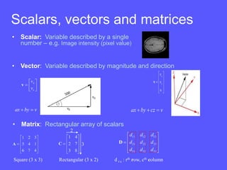
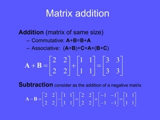
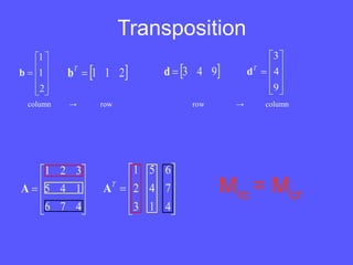
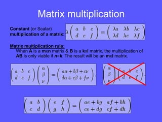
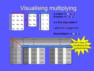
This document provides an overview of matrix algebra concepts including: - Matrices are rectangular arrays of scalars that are defined by their number of rows and columns. Common matrix operations include addition, subtraction, multiplication, and transposition. - Matrix multiplication involves multiplying the rows of the first matrix by the columns of the second, and can only be done if the number of columns of the first equals the number of rows of the second. 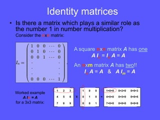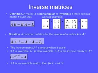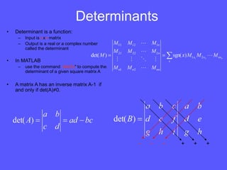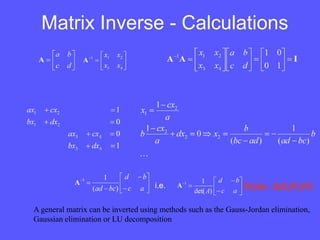- Identity matrices play a similar role to the number 1 in regular multiplication. The determinant of a matrix is a single number that can be used to determine if a matrix is invertible. 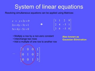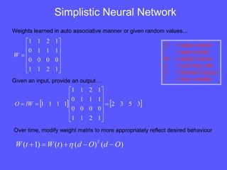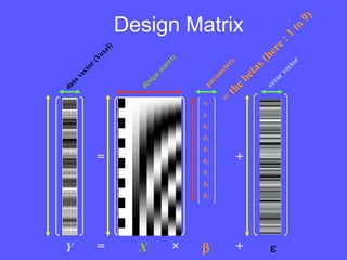- Example applications of matrix algebra include solving systems of linear equations, simple neural networks, and general linear

1. Matrix Algebra
Methods for Dummies
FIL
January 25 2006
Jon Machtynger & Jen Marchant

2. Acknowledgements / Info
• Mikkel Walletin’s (Excellent) slides
• John Ashburner (GLM context)
• Slides from SPM courses:
http://www.fil.ion.ucl.ac.uk/spm/course/
• Good Web Guides
– www.sosmath.com
– http://mathworld.wolfram.com/LinearAlgebra.html
– http://ceee.rice.edu/Books/LA/contents.html
– http://archives.math.utk.edu/topics/linearAlgebra.html

3. Scalars, vectors and matrices
• Scalar: Variable described by a single
number – e.g. Image intensity (pixel value)
• Vector: Variable described by magnitude and direction
Square (3 x 3) Rectangular (3 x 2) d r c : rth row, cth column
3
2
• Matrix: Rectangular array of scalars

4. Matrices
• A matrix is defined by the number of Rows and the
number of Columns.
• An mxn matrix has m rows and n columns.
A = 4x3 matrix
• A square matrix of order n, is an nxn matrix.
21 2 53
5 34 12
6 33 55
74 27 3
Matlab notes ( ;  End of matrix row )
A = [ 21 5 53 ; 5 34 12 ; 6 33 55 ; 74 27 3 ]
To extract data: Matrix name( row, column )
Scalar Data Point A( 1 , 2 ) = 2
Row Vector A( 2 , : ) = [ 5 34 12 ]
Column Vector A( : , 3 ) = [ 53 ; 12 ; 55 ; 3 ]
Smaller Matrix A(2:4,1:2) = [ 5 34 ; 6 33 ; 74 27 ]
Another Matrix A( 2:2:4 , 2:3 ) = [ 34 12 ; 27 3 ]

5. Addition (matrix of same size)
– Commutative: A+B=B+A
– Associative: (A+B)+C=A+(B+C)
Subtraction consider as the addition of a negative matrix
Matrix addition

6. Matrix multiplication
Matrix multiplication rule:
When A is a mxn matrix & B is a kxl matrix, the multiplication of
AB is only viable if n=k. The result will be an mxl matrix.
Constant (or Scalar)
multiplication of a matrix:

7. Visualising multiplying
b11 b12
b21 b22
b31 b32
a11 a12 a13 a11b11 + a12b21 + a13b31 a11b12 + a12b22 + a13b32
a21 a22 a23 a21b11 + a22b21 + a23b31 a21b12 + a22b22 + a23b32
a31 a32 a33 a31b11 + a32b21 + a33b31 a31b12 + a32b22 + a33b32
a41 a42 a43 a41b11 + a42b21 + a43b31 a41b12 + a42b22 + a43b32
a11 a12 a13 b11 b12 ? ?
a21 a22 a23 X b21 b22 = ? ?
a31 a32 a33 b31 b32 ? ?
a41 a42 a43 ? ?
A matrix = ( m x n )
B matrix = ( k x l )
A x B is only viable if
k = n
width of A = height of B
Result Matrix = ( m x l )
Jen’s way of
visualising the
multiplication

8. Transposition
column → row row → column
Mrc = Mcr

9. Outer product = matrix
Inner product = scalar
Two vectors:
Example
Note: (1xn)(nx1)  (1X1)
Note: (nx1)(1xn)  (nXn)

10. Identity matrices
• Is there a matrix which plays a similar role as
the number 1 in number multiplication?
Consider the nxn matrix:
A square nxn matrix A has one
A In = In A = A
An nxm matrix A has two!!
In A = A & A Im = A
1 2 3 1 0 0 1+0+0 0+2+0 0+0+3
4 5 6 X 0 1 0 = 4+0+0 0+5+0 0+0+6
7 8 9 0 0 1 7+0+0 0+8+0 0+0+9
Worked example
A In = A
for a 3x3 matrix:

11. Inverse matrices
• Definition. A matrix A is nonsingular or invertible if there exists a
matrix B such that: worked example:
• Notation. A common notation for the inverse of a matrix A is A-1.
• If A is an invertible matrix, then (AT)-1 = (A-1)T
• The inverse matrix A-1 is unique when it exists.
• If A is invertible, A-1 is also invertible  A is the inverse matrix of A-1.
1 1 X
2
3
-1
3
=
2 + 1
3 3
-1 + 1
3 3
= 1 0
-1 2
1
3
1
3
-2+ 2
3 3
1 + 2
3 3
0 1

12. Determinants
• Determinant is a function:
– Input is nxn matrix
– Output is a real or a complex number
called the determinant
• In MATLAB
– use the command det(A)" to compute the
determinant of a given square matrix A
• A matrix A has an inverse matrix A-1 if
and only if det(A)≠0.
+ + +
- - -

13. Matrix Inverse - Calculations
A general matrix can be inverted using methods such as the Gauss-Jordan elimination,
Gaussian elimination or LU decomposition
i.e. Note: det(A)≠0

14. Some Application Areas

15. Some Application Areas
• Simultaneous Equations
• Simple Neural Network
• GLM

16. System of linear equations
Resolving simultaneous equations can be applied using Matrices:
• Multiply a row by a non-zero constant
• Interchange two rows
• Add a multiple of one row to another row

…
Also known as
Gaussian Elimination

17. Simplistic Neural Network
O = output vector
I = input vector
W = weight matrix
η = Learning rate
d = Desired output
t = time variable
Given an input, provide an output…
Weights learned in auto associative manner or given random values…
Over time, modify weight matrix to more appropriately reflect desired behaviour

18. a
m
b3
b4
b5
b6
b7
b8
b9
+
e
= b +
Y X ×
Design Matrix
=

19. a
m
b3
b4
b5
b6
b7
b8
b9
+
e
= b +
Y X ×
Design Matrix
=

20. Questions?