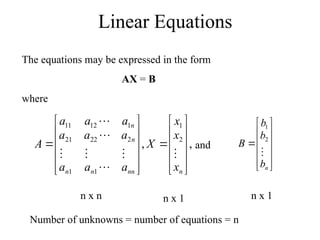
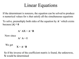
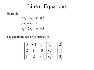
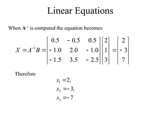
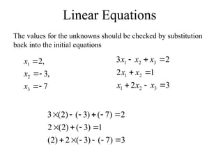
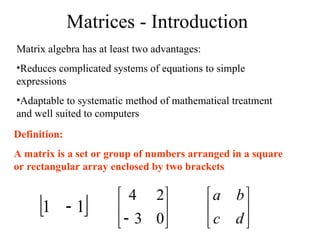
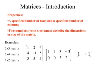
The document provides an introduction to matrices, including their definitions, properties, and various operations such as addition, subtraction, and multiplication. It discusses matrix dimensions, the use of determinants for matrix inversion, and the concepts of minors and cofactors. Additionally, it explains the importance of matrices in solving linear equations, particularly in the context of survey problems.

1. Matrices
Introduction

2. Matrices - Introduction
Matrix algebra has at least two advantages:
•Reduces complicated systems of equations to simple
expressions
•Adaptable to systematic method of mathematical treatment
and well suited to computers
Definition:
A matrix is a set or group of numbers arranged in a square
or rectangular array enclosed by two brackets
 
1
1  





 0
3
2
4






d
c
b
a

3. Matrices - Introduction
Properties:
•A specified number of rows and a specified number of
columns
•Two numbers (rows x columns) describe the dimensions
or size of the matrix.
Examples:
3x3 matrix
2x4 matrix
1x2 matrix











3
3
3
5
1
4
4
2
1





 
2
3
3
3
0
1
0
1
 
1
1 

4. Matrices - Introduction
A matrix is denoted by a bold capital letter and the elements
within the matrix are denoted by lower case letters
e.g. matrix [A] with elements aij














mn
ij
m
m
n
ij
in
ij
a
a
a
a
a
a
a
a
a
a
a
a
2
1
2
22
21
12
11
...
...




i goes from 1 to m
j goes from 1 to n
Amxn=
mAn

5. Matrices
Matrix Operations

6. Matrices - Operations
ADDITION AND SUBTRACTION OF MATRICES
The sum or difference of two matrices, A and B of the same
size yields a matrix C of the same size
ij
ij
ij b
a
c 

Matrices of different sizes cannot be added or subtracted

7. Matrices - Operations
MULTIPLICATION OF MATRICES
The product of two matrices is another matrix
Two matrices A and B must be conformable for multiplication
to be possible
i.e. the number of columns of A must equal the number of rows
of B
Example.
A x B = C
(1x3) (3x1) (1x1)

8. Matrices - Operations























22
21
12
11
32
31
22
21
12
11
23
22
21
13
12
11
c
c
c
c
b
b
b
b
b
b
a
a
a
a
a
a
22
32
23
22
22
12
21
21
31
23
21
22
11
21
12
32
13
22
12
12
11
11
31
13
21
12
11
11
)
(
)
(
)
(
)
(
)
(
)
(
)
(
)
(
)
(
)
(
)
(
)
(
c
b
a
b
a
b
a
c
b
a
b
a
b
a
c
b
a
b
a
b
a
c
b
a
b
a
b
a
























Successive multiplication of row i of A with column j of
B – row by column multiplication

9. Matrices - Operations











































)
3
7
(
)
2
2
(
)
8
4
(
)
5
7
(
)
6
2
(
)
4
4
(
)
3
3
(
)
2
2
(
)
8
1
(
)
5
3
(
)
6
2
(
)
4
1
(
3
5
2
6
8
4
7
2
4
3
2
1







57
63
21
31
Remember also:
IA = A






1
0
0
1






57
63
21
31







57
63
21
31

10. Matrices - Operations
Assuming that matrices A, B and C are conformable for
the operations indicated, the following are true:
1. AI = IA = A
2. A(BC) = (AB)C = ABC - (associative law)
3. A(B+C) = AB + AC - (first distributive law)
4. (A+B)C = AC + BC - (second distributive law)
Caution!
1. AB not generally equal to BA, BA may not be conformable
2. If AB = 0, neither A nor B necessarily = 0
3. If AB = AC, B not necessarily = C

11. Matrices - Operations
AB not generally equal to BA, BA may not be conformable






















































0
10
6
23
0
5
2
1
2
0
4
3
20
15
8
3
2
0
4
3
0
5
2
1
2
0
4
3
0
5
2
1
ST
TS
S
T

12. Matrices - Operations
If AB = 0, neither A nor B necessarily = 0





















0
0
0
0
3
2
3
2
0
0
1
1

13. Matrices - Operations
TRANSPOSE OF A MATRIX
If :








1
3
5
7
4
2
3
2 A
A
2x3












1
7
3
4
5
2
3
2
T
T
A
A
Then transpose of A, denoted AT
is:
T
ji
ij a
a  For all i and j

14. Matrices - Operations
Properties of transposed matrices:
1. (A+B)T
= AT
+ BT
2. (AB)T
= BT
AT
3. (kA)T
= kAT
4. (AT
)T
= A

15. Matrices - Operations
SYMMETRIC MATRICES
A Square matrix is symmetric if it is equal to its
transpose:
A = AT














d
b
b
a
A
d
b
b
a
A
T

16. Matrices - Operations
INVERSE OF A MATRIX
Consider a scalar k. The inverse is the reciprocal or division of 1
by the scalar.
Example:
k=7 the inverse of k or k-1
= 1/k = 1/7
Division of matrices is not defined since there may be AB = AC
while B = C
Instead matrix inversion is used.
The inverse of a square matrix, A, if it exists, is the unique matrix
A-1
where:
AA-1
= A-1
A = I

17. Matrices - Operations
Example:


















3
2
1
1
1
2
1
3
1
2
2
A
A
A










































1
0
0
1
3
2
1
1
1
2
1
3
1
0
0
1
1
2
1
3
3
2
1
1
Because:

18. Matrices - Operations
Properties of the inverse:
1
1
1
1
1
1
1
1
1
1
)
(
)
(
)
(
)
(
)
(













A
k
kA
A
A
A
A
A
B
AB
T
T
A square matrix that has an inverse is called a nonsingular matrix
A matrix that does not have an inverse is called a singular matrix
Square matrices have inverses except when the determinant is zero
When the determinant of a matrix is zero the matrix is singular

19. Matrices - Operations
DETERMINANT OF A MATRIX
To compute the inverse of a matrix, the determinant is required
Each square matrix A has a unit scalar value called the
determinant of A, denoted by det A or |A|
5
6
2
1
5
6
2
1








A
A
If
then

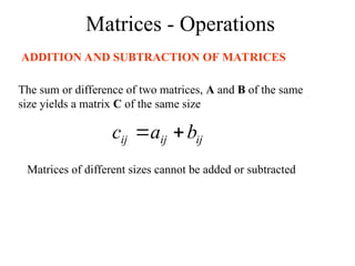
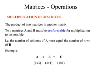
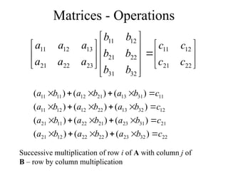
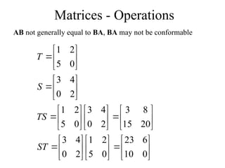
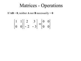
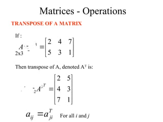
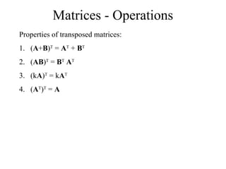
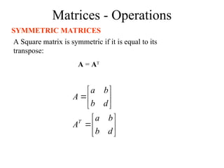
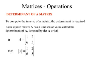
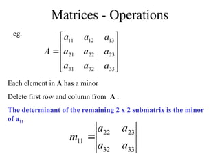
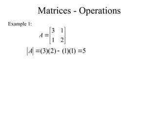
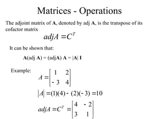
20. Matrices - Operations
If A = [A] is a single element (1x1), then the determinant is
defined as the value of the element
Then |A| =det A = a11
If A is (n x n), its determinant may be defined in terms of order
(n-1) or less.

21. Matrices - Operations
MINORS
If A is an n x n matrix and one row and one column are deleted,
the resulting matrix is an (n-1) x (n-1) submatrix of A.
The determinant of such a submatrix is called a minor of A and
is designated by mij , where i and j correspond to the deleted
row and column, respectively.
mij is the minor of the element aij in A.

22. Matrices - Operations











33
32
31
23
22
21
13
12
11
a
a
a
a
a
a
a
a
a
A
Each element in A has a minor
Delete first row and column from A .
The determinant of the remaining 2 x 2 submatrix is the minor
of a11
eg.
33
32
23
22
11
a
a
a
a
m 

23. Matrices - Operations
Therefore the minor of a12 is:
And the minor for a13 is:
33
31
23
21
12
a
a
a
a
m 
32
31
22
21
13
a
a
a
a
m 

24. Matrices - Operations
COFACTORS
The cofactor Cij of an element aij is defined as:
ij
j
i
ij m
C 

 )
1
(
When the sum of a row number i and column j is even, cij = mij and
when i+j is odd, cij =-mij
13
13
3
1
13
12
12
2
1
12
11
11
1
1
11
)
1
(
)
3
,
1
(
)
1
(
)
2
,
1
(
)
1
(
)
1
,
1
(
m
m
j
i
c
m
m
j
i
c
m
m
j
i
c






















25. Matrices - Operations
Therefore the 2 x 2 matrix :







22
21
12
11
a
a
a
a
A
Has cofactors :
22
22
11
11 a
a
m
c 


And:
21
21
12
12 a
a
m
c 





And the determinant of A is:
21
12
22
11
12
12
11
11 a
a
a
a
c
a
c
a
A 




26. Matrices - Operations
Example 1:







2
1
1
3
A
5
)
1
)(
1
(
)
2
)(
3
( 


A

27. Matrices - Operations
For a 3 x 3 matrix:











33
32
31
23
22
21
13
12
11
a
a
a
a
a
a
a
a
a
A
The cofactors of the first row are:
31
22
32
21
32
31
22
21
13
31
23
33
21
33
31
23
21
12
32
23
33
22
33
32
23
22
11
)
(
a
a
a
a
a
a
a
a
c
a
a
a
a
a
a
a
a
c
a
a
a
a
a
a
a
a
c












28. Matrices - Operations
The determinant of a matrix A is:
21
12
22
11
12
12
11
11 a
a
a
a
c
a
c
a
A 



Which by substituting for the cofactors in this case is:
)
(
)
(
)
( 31
22
32
21
13
31
23
33
21
12
32
23
33
22
11 a
a
a
a
a
a
a
a
a
a
a
a
a
a
a
A 






29. Matrices - Operations
ADJOINT MATRICES
A cofactor matrix C of a matrix A is the square matrix of the same
order as A in which each element aij is replaced by its cofactor cij .
Example:








4
3
2
1
A








1
2
3
4
C
If
The cofactor C of A is

30. Matrices - Operations
The adjoint matrix of A, denoted by adj A, is the transpose of its
cofactor matrix
T
C
adjA 
It can be shown that:
A(adj A) = (adjA) A = |A| I
Example:





 














1
3
2
4
10
)
3
)(
2
(
)
4
)(
1
(
4
3
2
1
T
C
adjA
A
A

31. Matrices - Operations
USING THE ADJOINT MATRIX IN MATRIX INVERSION
A
adjA
A 
 1
Since
AA-1
= A-1
A = I
and
A(adj A) = (adjA) A = |A| I
then

32. Matrices and Linear Equations
Linear Equations

33. Linear Equations
Linear equations are common and important for survey
problems
Matrices can be used to express these linear equations and
aid in the computation of unknown values
Example
n equations in n unknowns, the aij are numerical coefficients,
the bi are constants and the xj are unknowns
n
n
nn
n
n
n
n
n
n
b
x
a
x
a
x
a
b
x
a
x
a
x
a
b
x
a
x
a
x
a
















2
2
1
1
2
2
2
22
1
21
1
1
2
12
1
11

34. Linear Equations
The equations may be expressed in the form
AX = B
where
,
, 2
1
1
1
2
22
21
1
12
11


























n
nn
n
n
n
n
x
x
x
X
a
a
a
a
a
a
a
a
a
A







and













n
b
b
b
B

2
1
n x n n x 1 n x 1
Number of unknowns = number of equations = n

35. Linear Equations
If the determinant is nonzero, the equation can be solved to produce
n numerical values for x that satisfy all the simultaneous equations
To solve, premultiply both sides of the equation by A-1
which exists
because |A| = 0
A-1
AX = A-1
B
Now since
A-1
A = I
We get
X = A-1
B
So if the inverse of the coefficient matrix is found, the unknowns,
X would be determined

36. Linear Equations
Example
3
2
1
2
2
3
3
2
1
2
1
3
2
1








x
x
x
x
x
x
x
x
The equations can be expressed as

































3
1
2
1
2
1
0
1
2
1
1
3
3
2
1
x
x
x

37. Linear Equations
When A-1
is computed the equation becomes






































 
7
3
2
3
1
2
5
.
2
5
.
3
5
.
1
0
.
1
0
.
2
0
.
1
5
.
0
5
.
0
5
.
0
1
B
A
X
Therefore
7
,
3
,
2
3
2
1





x
x
x

38. Linear Equations
The values for the unknowns should be checked by substitution
back into the initial equations
3
2
1
2
2
3
3
2
1
2
1
3
2
1








x
x
x
x
x
x
x
x
3
)
7
(
)
3
(
2
)
2
(
1
)
3
(
)
2
(
2
2
)
7
(
)
3
(
)
2
(
3
















7
,
3
,
2
3
2
1





x
x
x