DEFINITIO
N
A matrix isa set or group of numbers arranged in a square or
rectangular array enclosed by two brackets
Example 1:
PROPERTIES:
A specified number of rows and a specified number of columns
Two numbers (rows x columns) describe the dimensions or
size of the matrix or we say order of the matrix.
[4 2
3 0]
3.
DEFINITIO
N
PROPERTIES:
A specified numberof rows and a specified number of columns
Two numbers (rows × columns) describe the dimensions or size of the matrix
or we say order of the matrix.
Example 2:
- 1 x 2 matrix (1 row, 2 columns)
- 2 x 2 matrix (1 row, 2 columns)
- 2 x 4 matrix (1 row, 2 columns)
[4 2
3 0]
4.
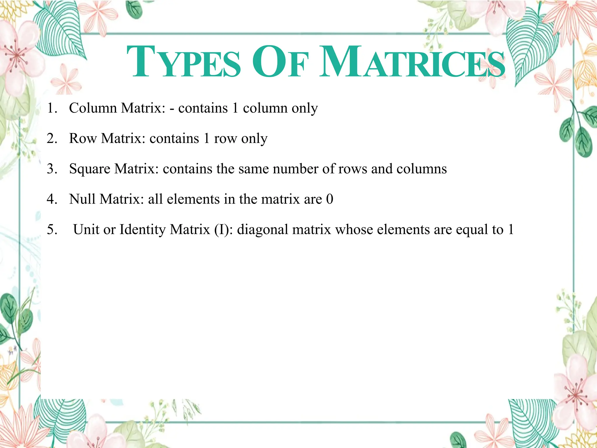
TYPES OF MATRICES
1.Column Matrix: - contains 1 column only
2. Row Matrix: contains 1 row only
3. Square Matrix: contains the same number of rows and columns
4. Null Matrix: all elements in the matrix are 0
5. Unit or Identity Matrix (I): diagonal matrix whose elements are equal to 1
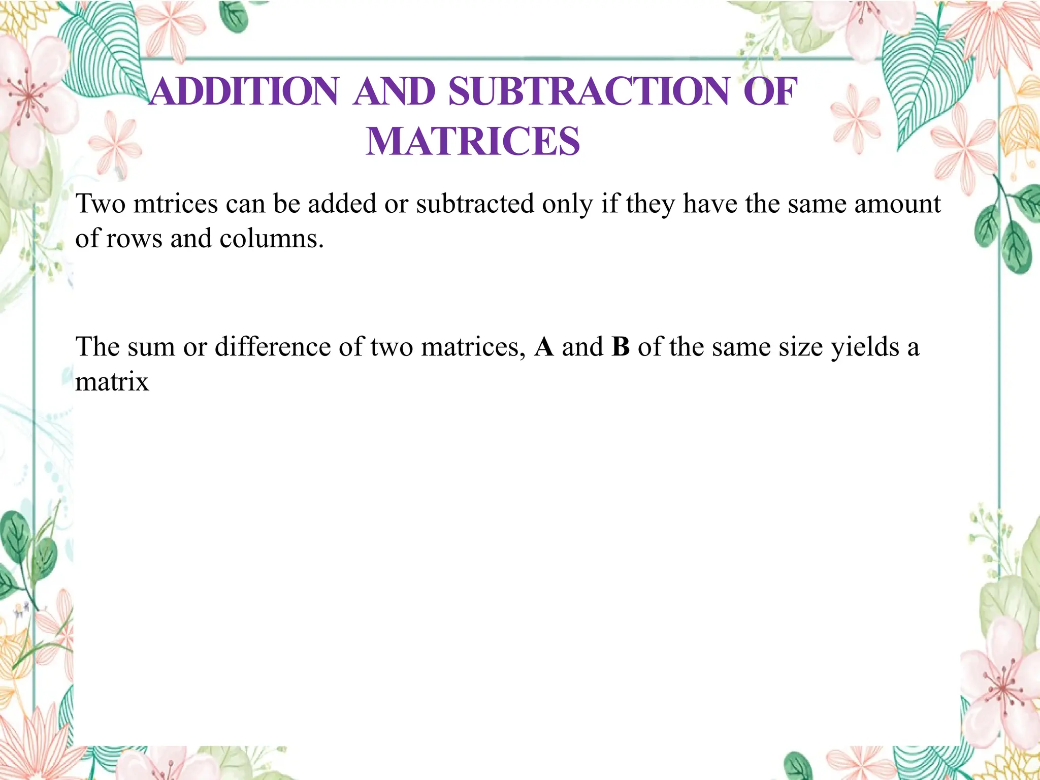
ADDITION AND SUBTRACTIONOF
MATRICES
Two mtrices can be added or subtracted only if they have the same amount
of rows and columns.
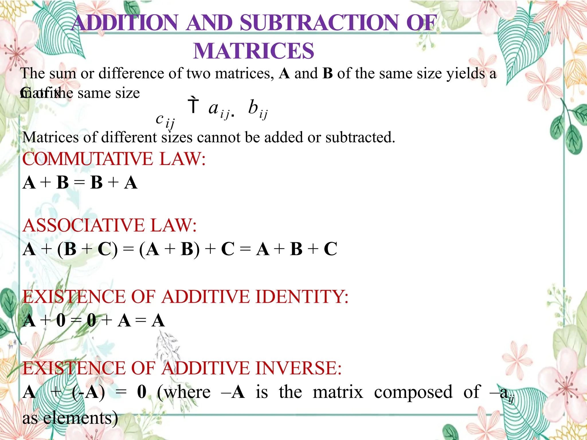
The sum or difference of two matrices, A and B of the same size yields a
matrix
7.
ADDITION AND SUBTRACTIONOF
MATRICES
The sum or difference of two matrices, A and B of the same size yields a
matrix
C of the same size
ai j bij
cij
Matrices of different sizes cannot be added or subtracted.
COMMUTATIVE LAW:
A + B = B + A
ASSOCIATIVE LAW:
A + (B + C) = (A + B) + C = A + B + C
EXISTENCE OF ADDITIVE IDENTITY:
A + 0 = 0 + A = A
EXISTENCE OF ADDITIVE INVERSE:
A + (-A) = 0 (where –A is the matrix composed of –aij
as elements)
8.
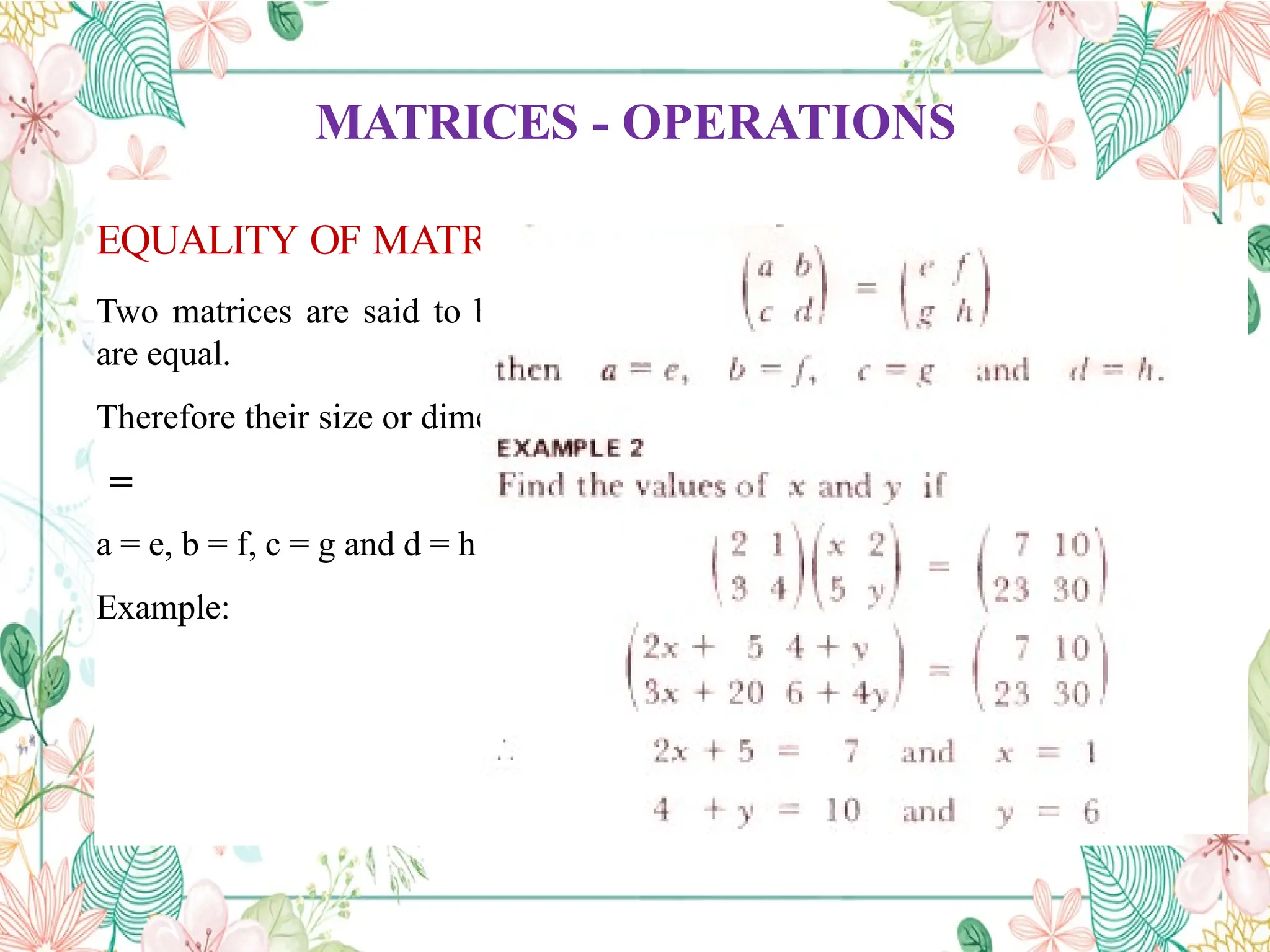
MATRICES - OPERATIONS
EQUALITYOF MATRICES
Two matrices are said to be equal only when all corresponding elements
are equal.
Therefore their size or dimensions are equal as well.
=
a = e, b = f, c = g and d = h
Example:
9.
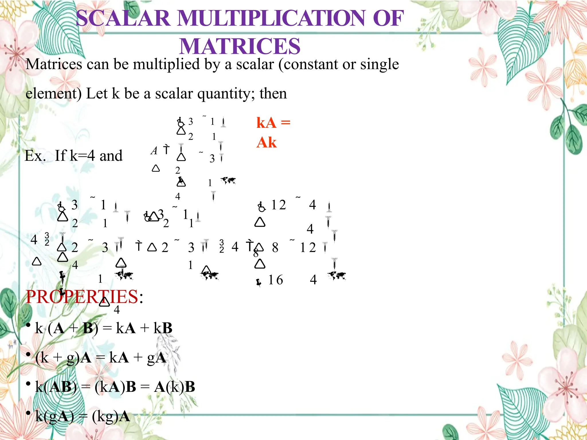
SCALAR MULTIPLICATION OF
MATRICES
Matricescan be multiplied by a scalar (constant or single
element) Let k be a scalar quantity; then
kA =
Ak
PROPERTIES:
• k (A + B) = kA + kB
• (k + g)A = kA + gA
• k(AB) = (kA)B = A(k)B
• k(gA) = (kg)A
Ex. If k=4 and
1
3
2
4
3 1
2 1
A
16 4
8 1 2
4
8
12 4
4
3 1
1
4
2 3 2 3
4 1
3 1
2 1 2 1
4
10.
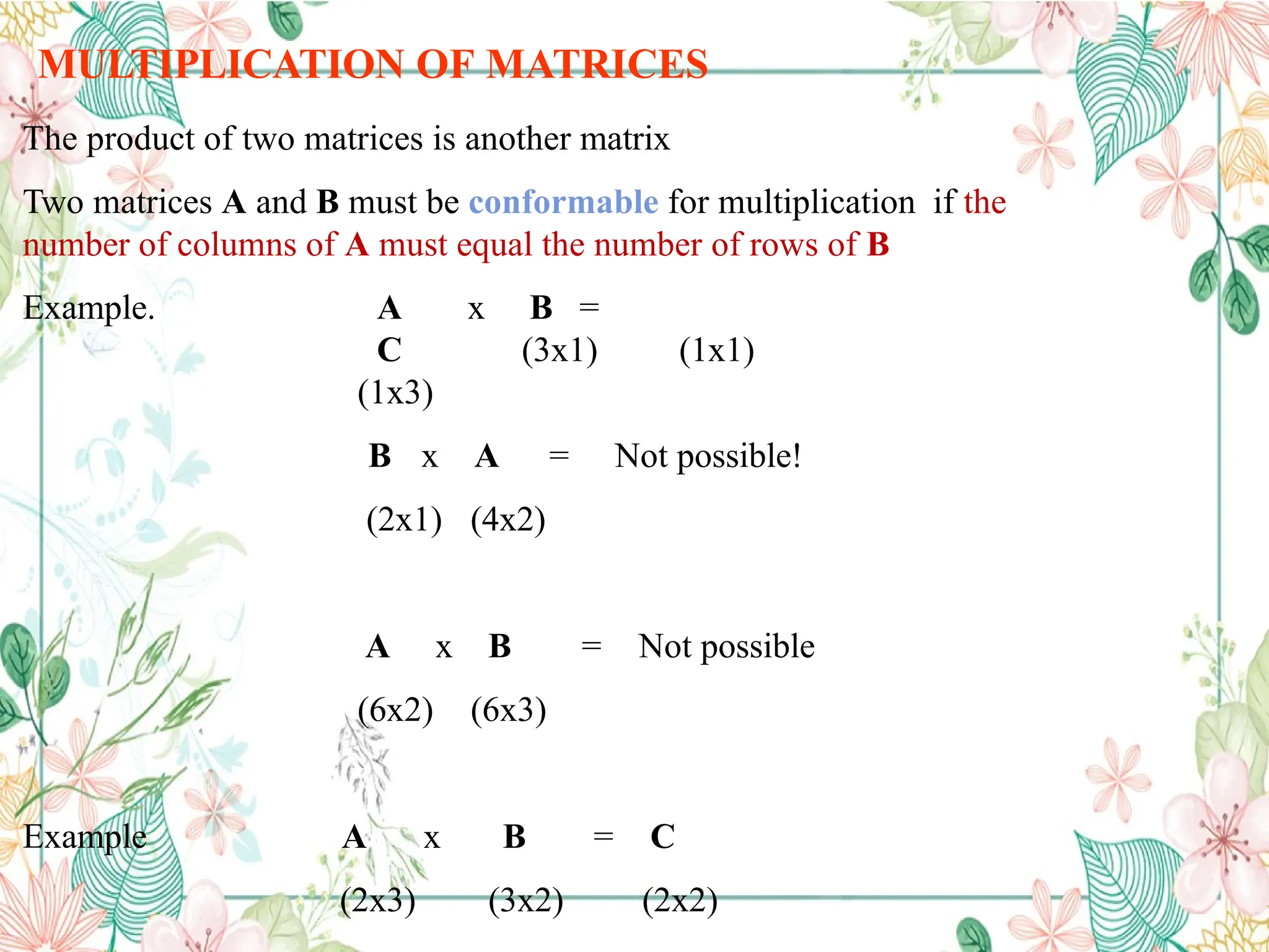
MULTIPLICATION OF MATRICES
Theproduct of two matrices is another matrix
Two matrices A and B must be conformable for multiplication if the
number of columns of A must equal the number of rows of B
Example. A x B =
C
(1x3)
(3x1) (1x1)
B x A
(2x1) (4x2)
= Not possible!
A x B
(6x2) (6x3)
= Not possible
Example A x B
(2x3) (3x2)
= C
(2x2)
11.
1 2
c 22
1 1
c
2 1
c
2 2
2 1
2 3
1 3
b31 b 3 2
a 2 2
1 2
1 1
a 2
1
a
c
b
b 1 2
b
b
1 1
a
a
a
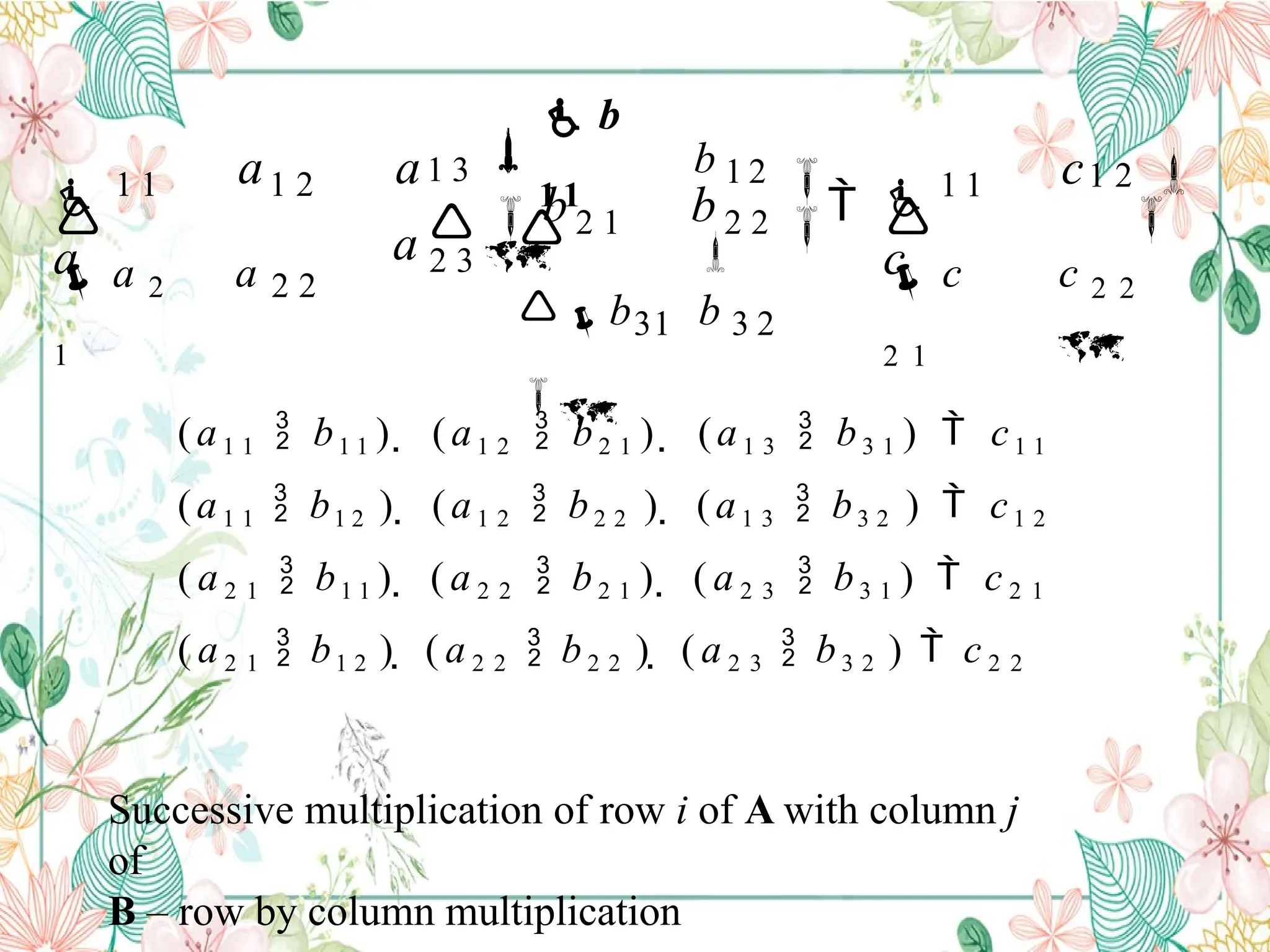
(a1 1 b1 1 ) (a1 2 b2 1 ) (a1 3 b3 1 ) c1 1
(a1 1 b1 2 ) (a1 2 b2 2 ) (a1 3 b3 2 ) c1 2
( a 2 1 b1 1 ) ( a 2 2 b2 1 ) ( a 2 3 b3 1 ) c 2 1
( a 2 1 b1 2 ) ( a 2 2 b2 2 ) ( a 2 3 b3 2 ) c 2 2
Successive multiplication of row i of A with column j
of
B – row by column multiplication
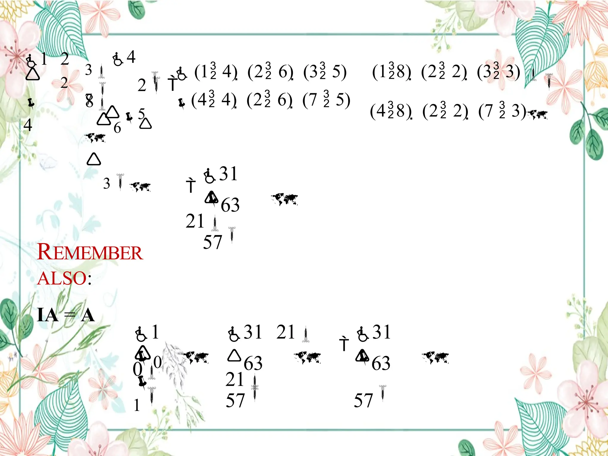
Assuming that matricesA, B and C are
conformable for the operations indicated, the following are
true:
1. AI = IA = A
2. A(BC) = (AB)C = ABC
3. A(B+C) = AB + AC
4. (A+B)C = AC + BC
- (existence of multiplicative identity)
- (associative law)
- (first distributive law)
- (second distributive law)
Caution!
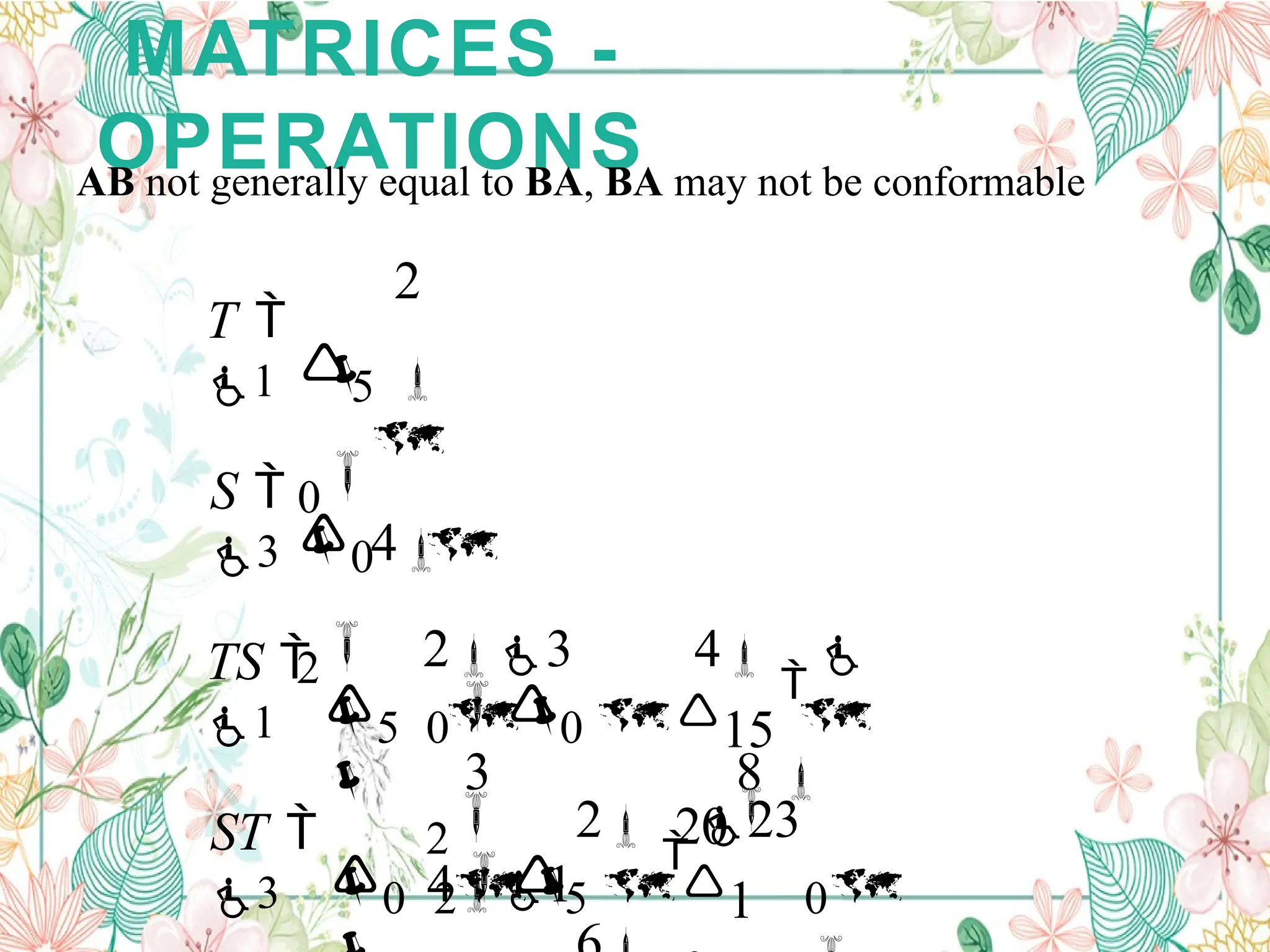
1. AB not generally equal to BA, BA may not be conformable
2. If AB = 0, neither A nor B necessarily = 0
3. If AB = AC, B not necessarily = C
PROPERTIES OF
MATRIX
MULTIPLICATION
14.
MATRICES -
OPERATIONS
AB notgenerally equal to BA, BA may not be conformable
0
1
2
23
0 25
41
15
20
5 00
2
23 4
3 8
0
2
4
5
0
2
ST
3
TS
1
S
3
T
1
15.
0 2
3
0 0
0
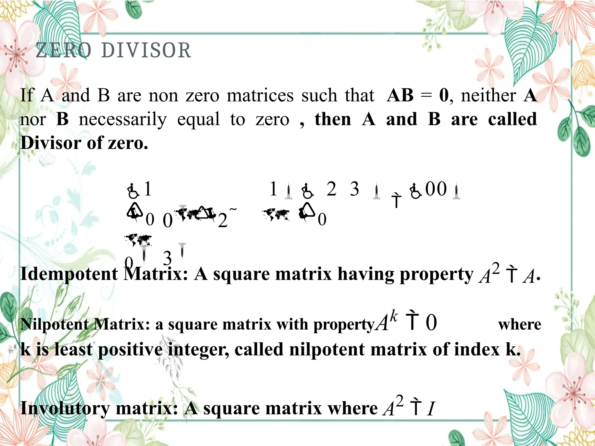
ZERO DIVISOR
If A and B are non zero matrices such that AB = 0, neither A
nor B necessarily equal to zero , then A and B are called
Divisor of zero.
1 1 2 3
00
Idempotent Matrix: A square matrix having property A2
A.
Nilpotent Matrix: a square matrix with propertyAk 0 where
k is least positive integer, called nilpotent matrix of index k.
Involutory matrix: A square matrix where A2
I
16.
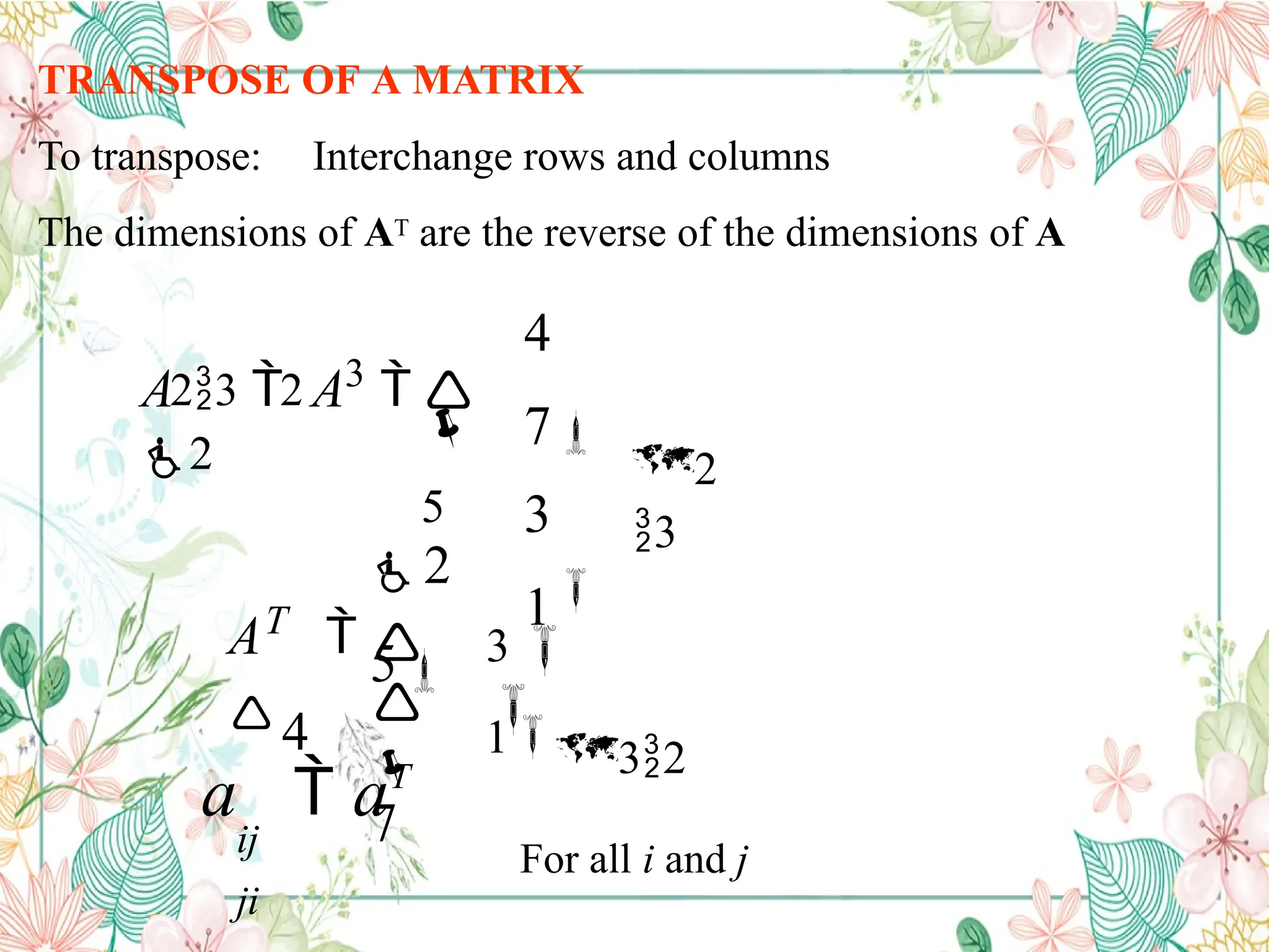
TRANSPOSE OF AMATRIX
To transpose: Interchange rows and columns
The dimensions of AT are the reverse of the dimensions of A
2
3
23 2
4
7
3
1
5
A A3
2
7
3
AT
4
2
5
132
For all i and j
a aT
ij
ji
17.
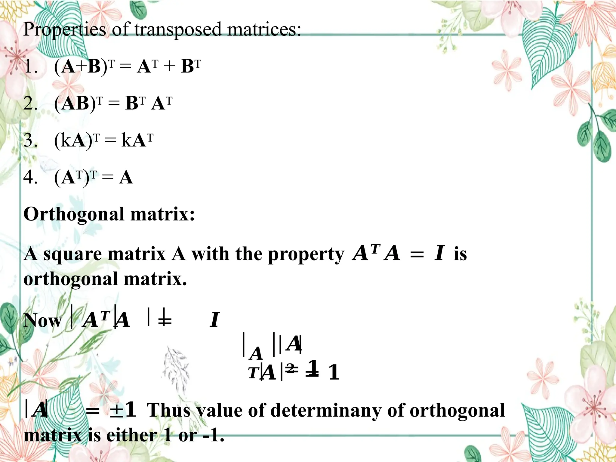
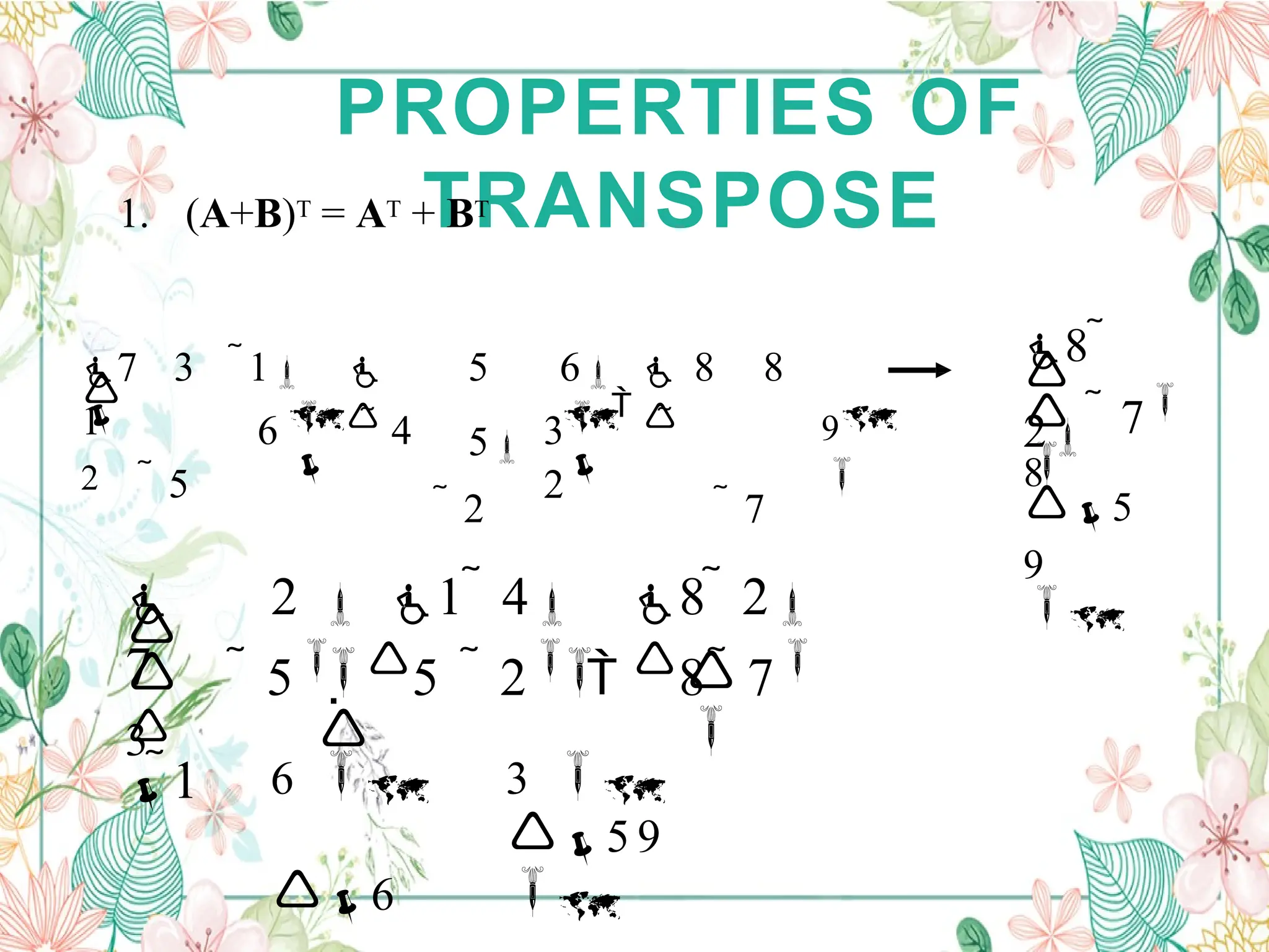
Properties of transposedmatrices:
1. (A+B)T = AT + BT
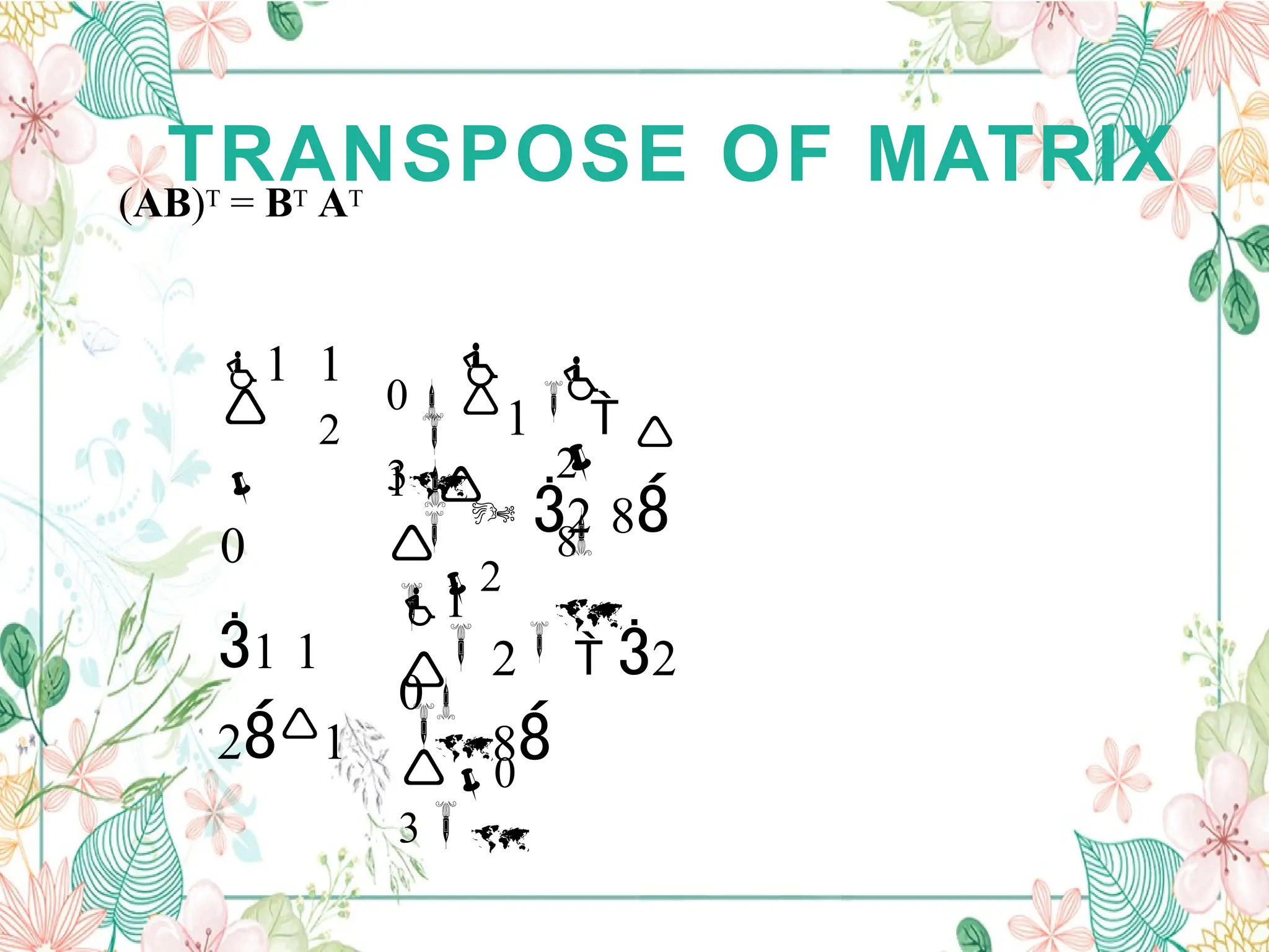
2. (AB)T = BT AT
3. (kA)T = kAT
4. (AT)T = A
Orthogonal matrix:
A square matrix A with the property 𝑨𝑻𝑨 = 𝑰 is
orthogonal matrix.
Now 𝑨𝑻
𝑨 = 𝑰
𝑨
𝑻
𝑨
= 𝟏
𝑨 𝟐 = 𝟏
𝑨 = ±𝟏 Thus value of determinany of orthogonal
matrix is either 1 or -1.
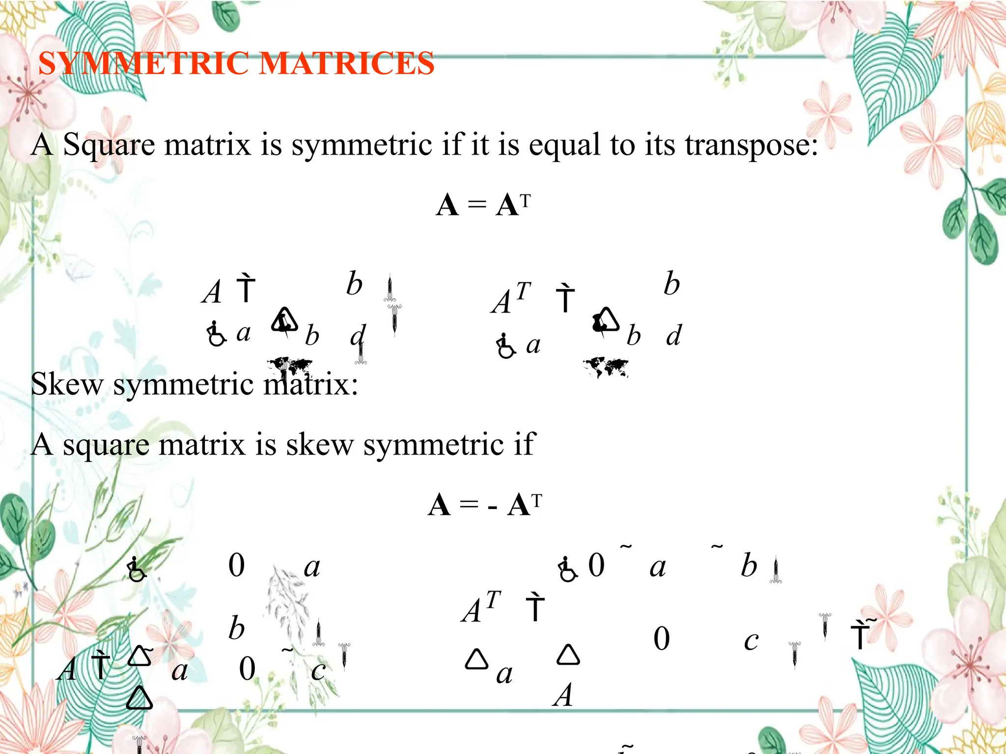
SYMMETRIC MATRICES
A Squarematrix is symmetric if it is equal to its transpose:
A = AT
Skew symmetric matrix:
A square matrix is skew symmetric if
A = - AT
b d b d
b b
A
a
AT
a
AT
a
0 a b
0 c
A
0 a
b
A a 0 c
21.
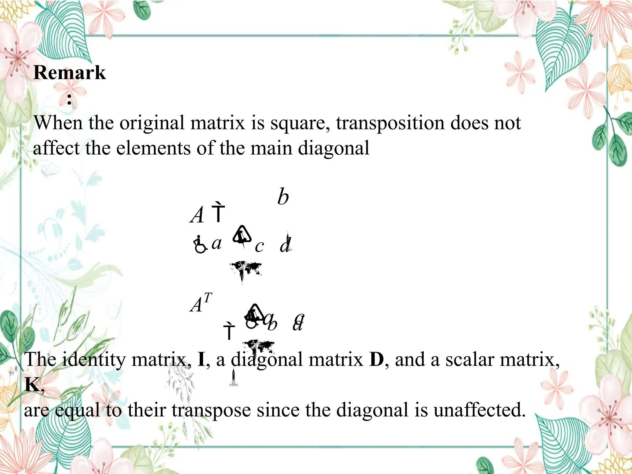
Remark
:
When the originalmatrix is square, transposition does not
affect the elements of the main diagonal
b d
a c
c d
b
A
a
AT
The identity matrix, I, a diagonal matrix D, and a scalar matrix,
K,
are equal to their transpose since the diagonal is unaffected.
22.
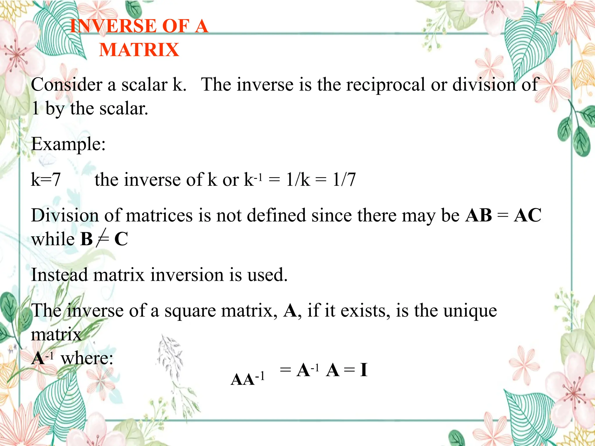
INVERSE OF A
MATRIX
Considera scalar k. The inverse is the reciprocal or division of
1 by the scalar.
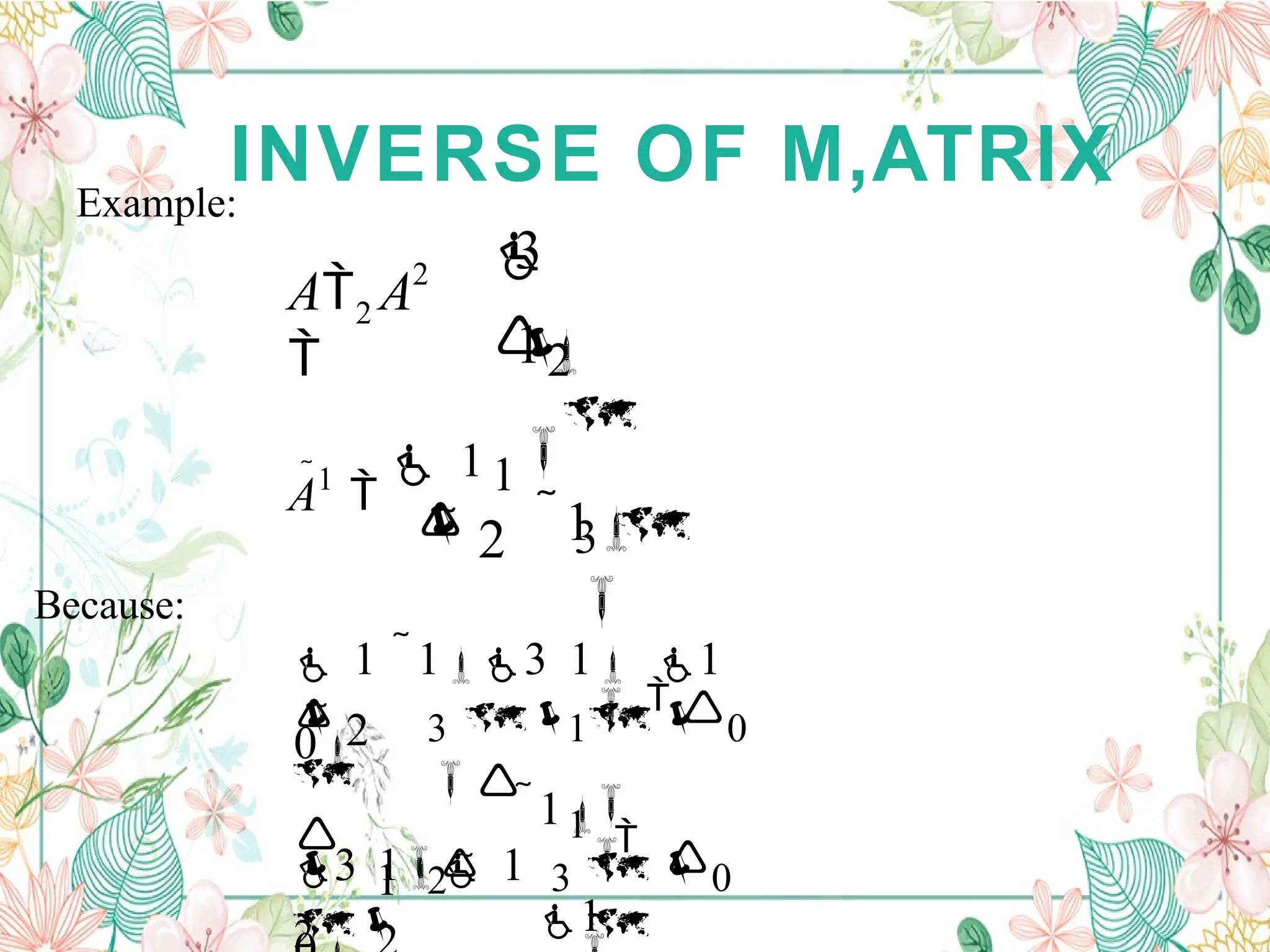
Example:
k=7 the inverse of k or k-1 = 1/k = 1/7
Division of matrices is not defined since there may be AB = AC
while B = C
Instead matrix inversion is used.
The inverse of a square matrix, A, if it exists, is the unique
matrix
A-1 where:
AA-1 = A-1 A = I
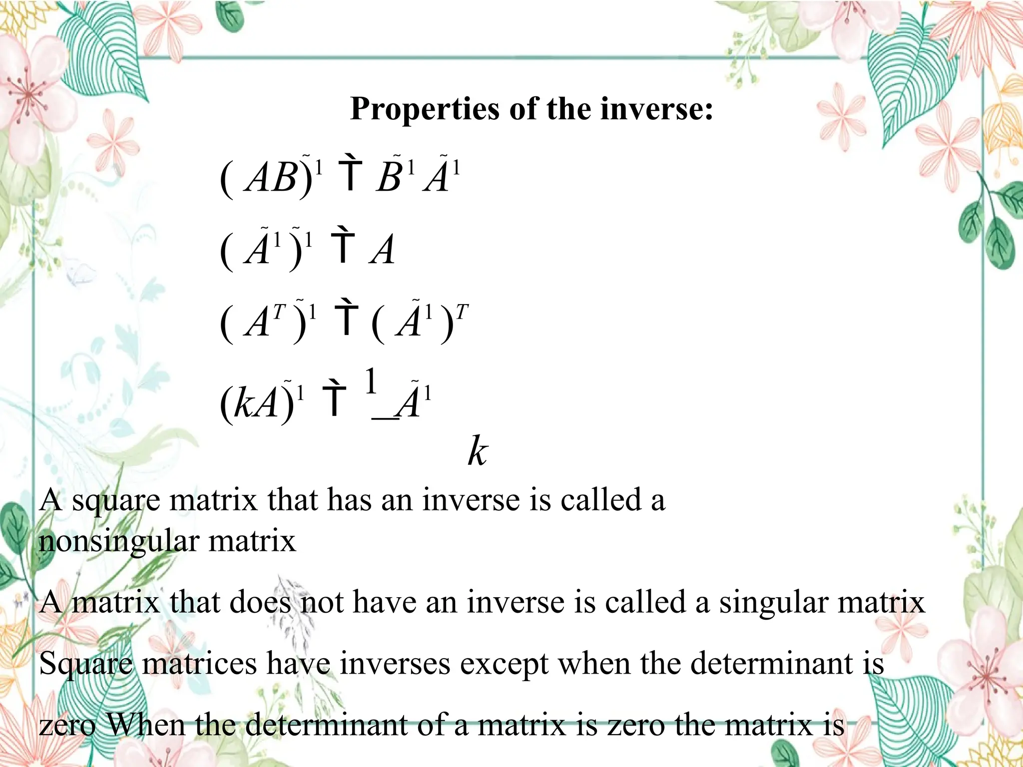
Properties of theinverse:
( AB)1
B1
A1
( A1
)1
A
( AT
)1
( A1
)T
(kA)1
1
A1
k
A square matrix that has an inverse is called a
nonsingular matrix
A matrix that does not have an inverse is called a singular matrix
Square matrices have inverses except when the determinant is
zero When the determinant of a matrix is zero the matrix is
25.
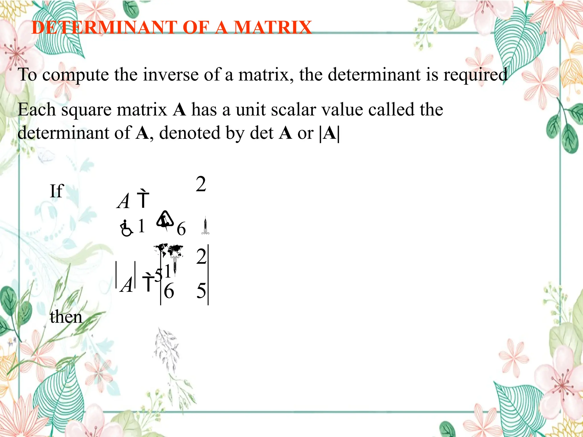
DETERMINANT OF AMATRIX
To compute the inverse of a matrix, the determinant is required
Each square matrix A has a unit scalar value called the
determinant of A, denoted by det A or |A|
2
6 5
2
6
5
A
1
A
1
If
then
26.
MATRICES - OPERATIONS
IfA = [A] is a single element (1x1), then the determinant
is defined as the value of the element
Then |A| =det A = a11
If A is (n x n), its determinant may be defined in terms of
order (n-1) or less.
27.
MATRICES -
OPERATIONS
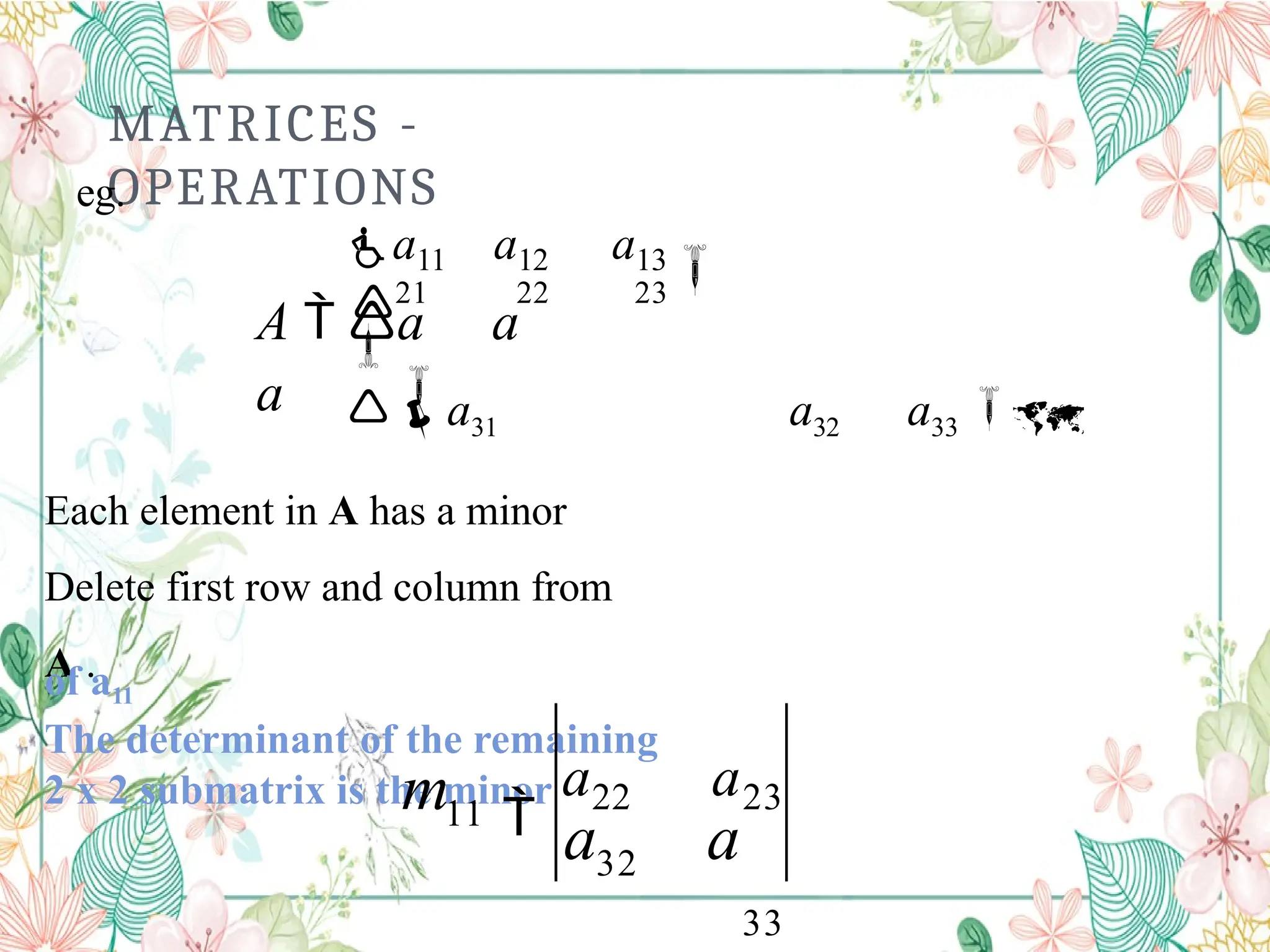
MINORS
If Ais an n x n matrix and one row and one column are deleted,
the resulting matrix is an (n-1) x (n-1) submatrix of A.
The determinant of such a submatrix is called a minor of A
and is designated by mij , where i and j correspond to the
deleted
row and column, respectively.
mij is the minor of the element aij in A.
28.
MATRICES -
OPERATIONS
21 2223
a11 a12 a13
A a a
a a31 a32 a33
Each element in A has a minor
Delete first row and column from
A .
The determinant of the remaining
2 x 2 submatrix is the minor
of a11
eg.
32
11
a a
a22 a23
33
m
29.
MATRICES - OPERATIONS
Thereforethe minor of a12 is:
And the minor for a13 is:
31
12
a a
a21 a23
33
m
31
13
a a
a21 a22
32
m
30.
MATRICES -
OPERATIONS
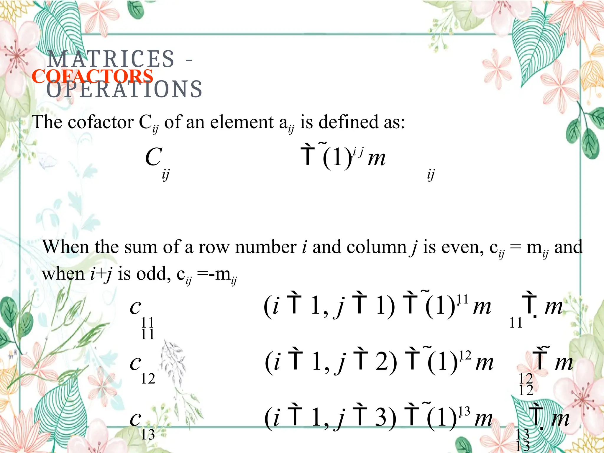
COFACTORS
The cofactorCij of an element aij is defined as:
C (1)i j
m
ij ij
When the sum of a row number i and column j is even, cij = mij and
when i+j is odd, cij =-mij
c (i 1, j 1) (1)11
m m
11 11
11
c (i 1, j 2) (1)12
m m
12 12
12
c (i 1, j 3) (1)13
m m
13 13
13
31.
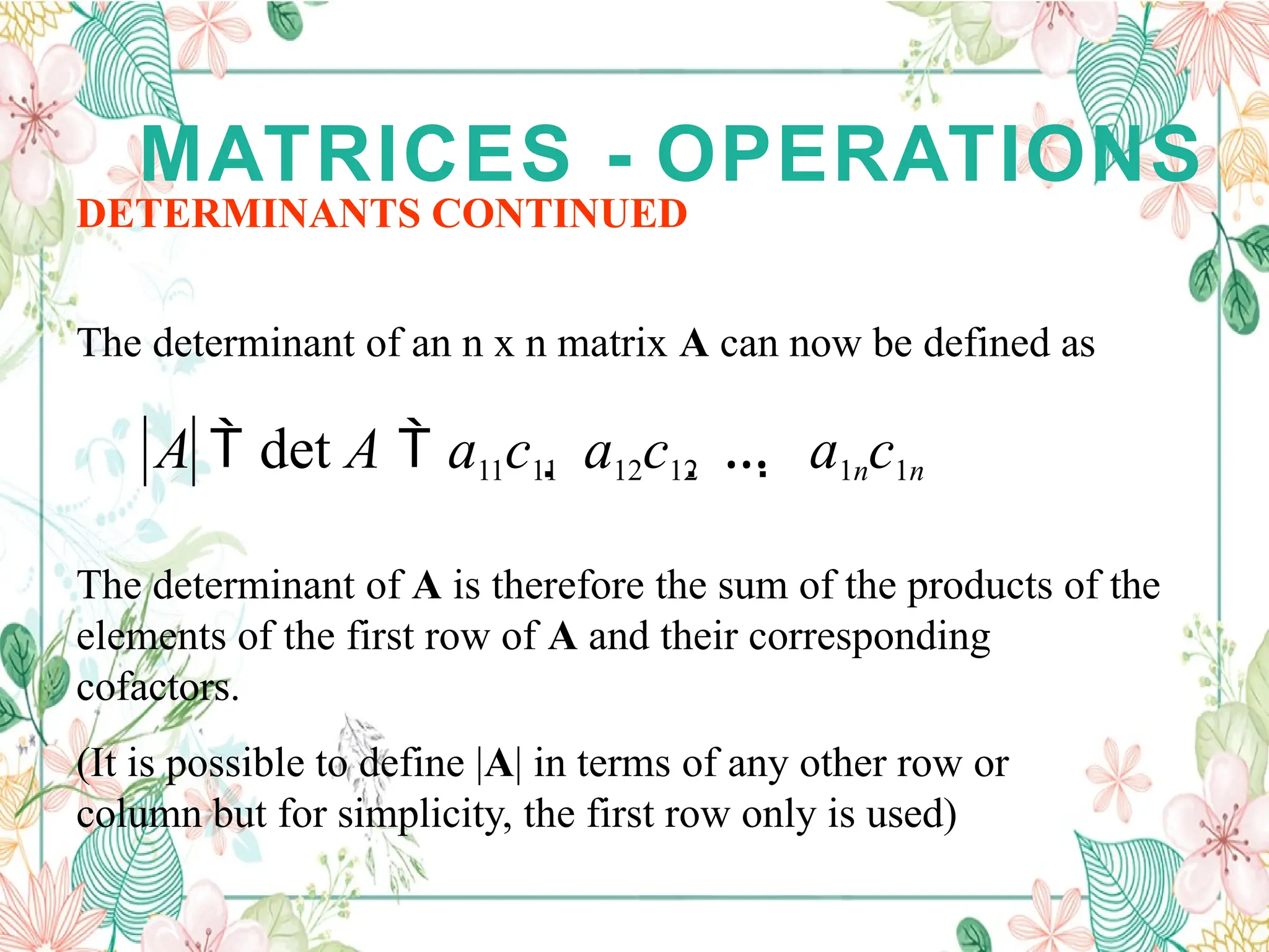
MATRICES - OPERATIONS
DETERMINANTSCONTINUED
The determinant of an n x n matrix A can now be defined as
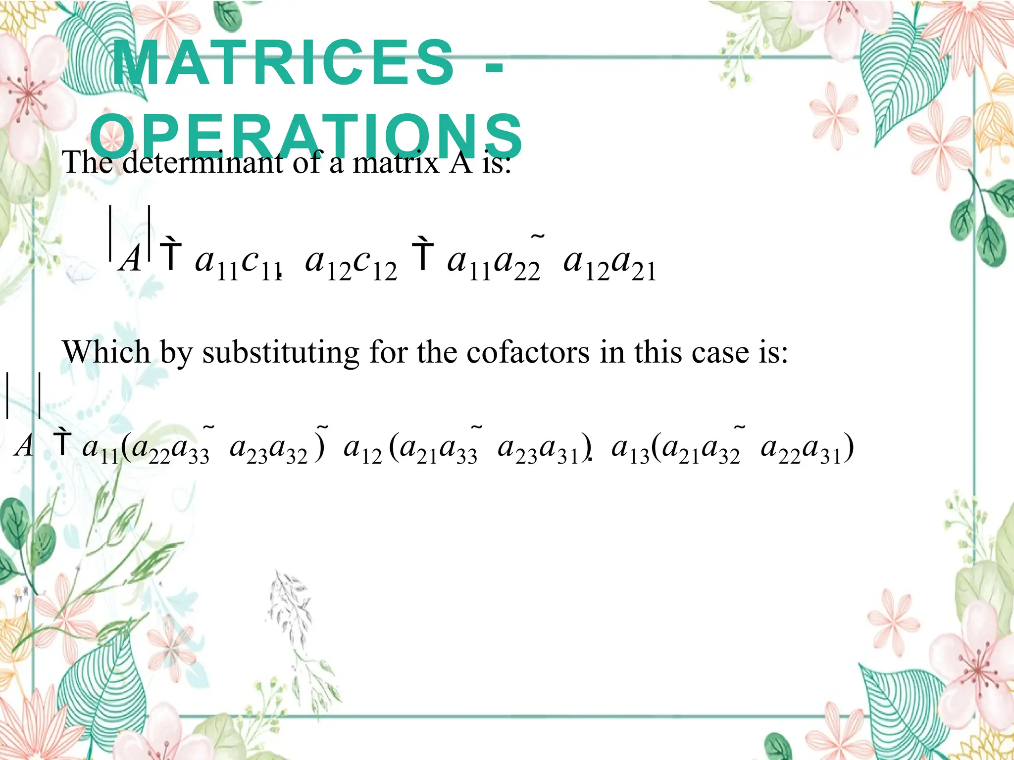
A det A a11c11 a12c12 … a1nc1n
The determinant of A is therefore the sum of the products of the
elements of the first row of A and their corresponding
cofactors.
(It is possible to define |A| in terms of any other row or
column but for simplicity, the first row only is used)
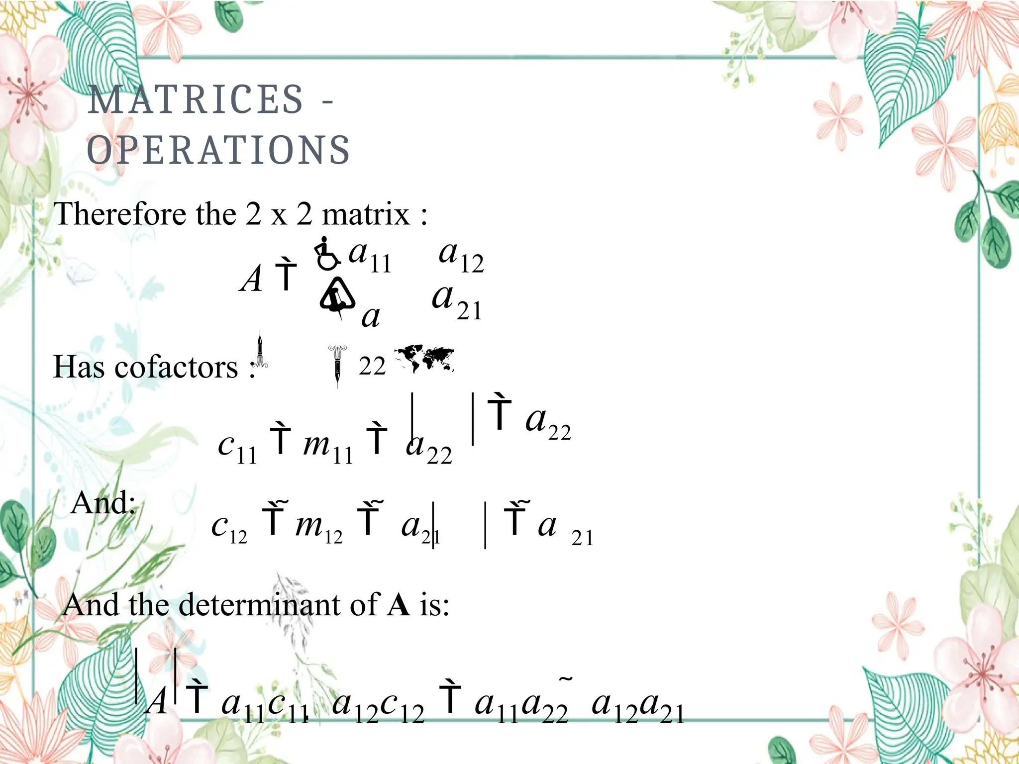
32.
MATRICES -
OPERATIONS
Therefore the2 x 2 matrix :
21
22
a
a
A
a11 a12
Has cofactors :
c11 m11 a22
a22
And:
21
c12 m12 a21 a
And the determinant of A is:
A a11c11 a12c12 a11a22 a12a21
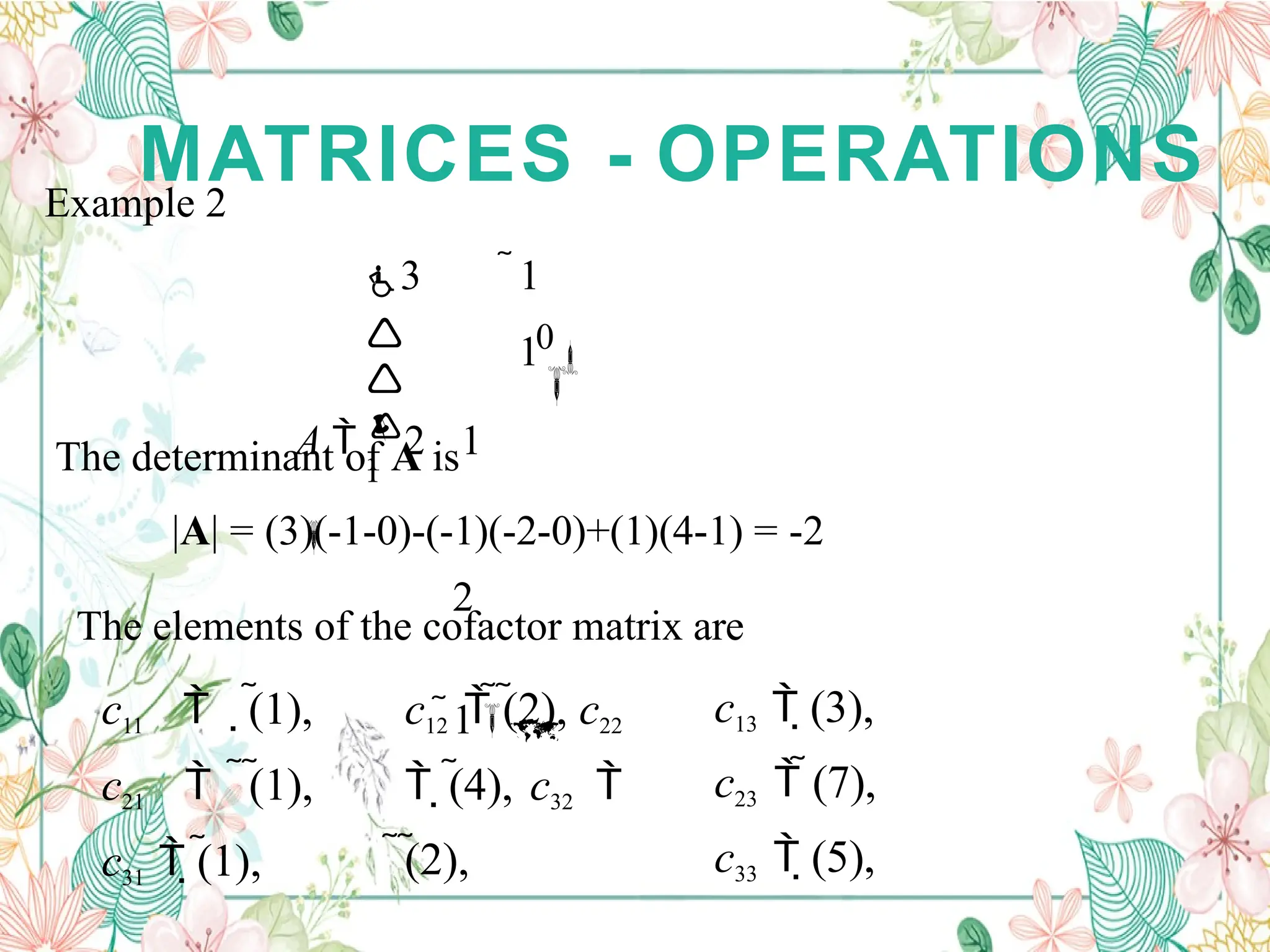
Fo
Mr a
A3
Tx
R3
Im
Ca
Etr
Six
-:
OPERATIONS
21 2223
a11 a12 a13
A a a
a a31
a32
a33
The cofactors of the first row are:
22 31
21 32
31
13
(a21a33 a23a31)
33
31
12
23 32
22 33
33
32
11
a a a a
a a
a21 a22
c
a a
a
a21 23
c
a a a a
a a
a
a22 23
c
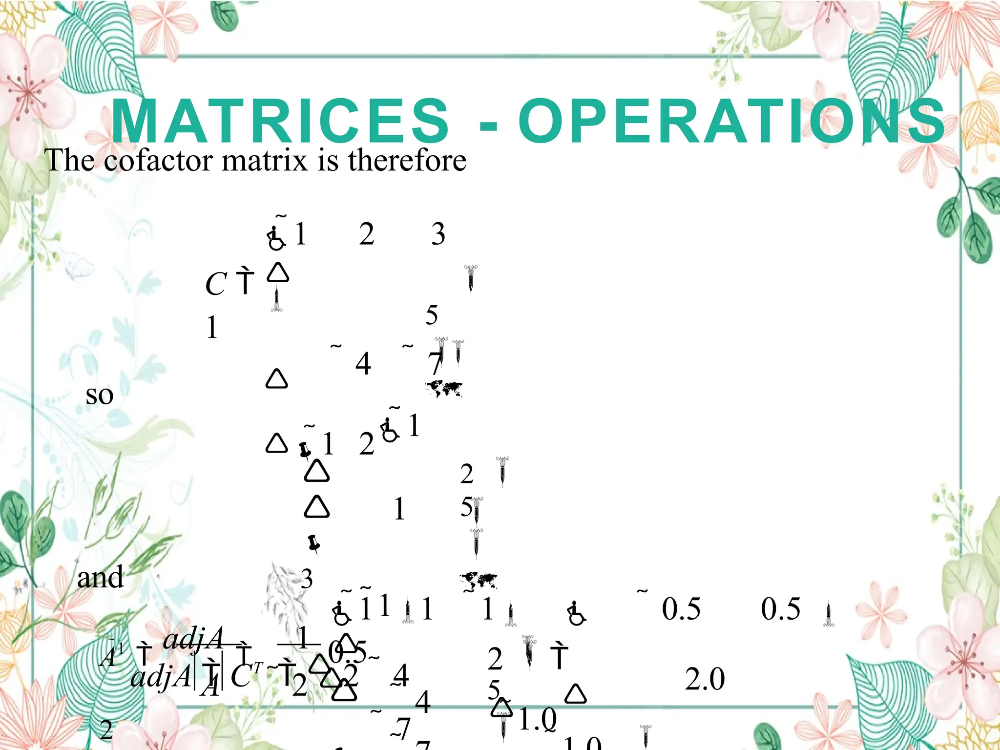
35.
MATRICES -
OPERATIONS
The determinantof a matrix A is:
A a11c11 a12c12 a11a22 a12a21
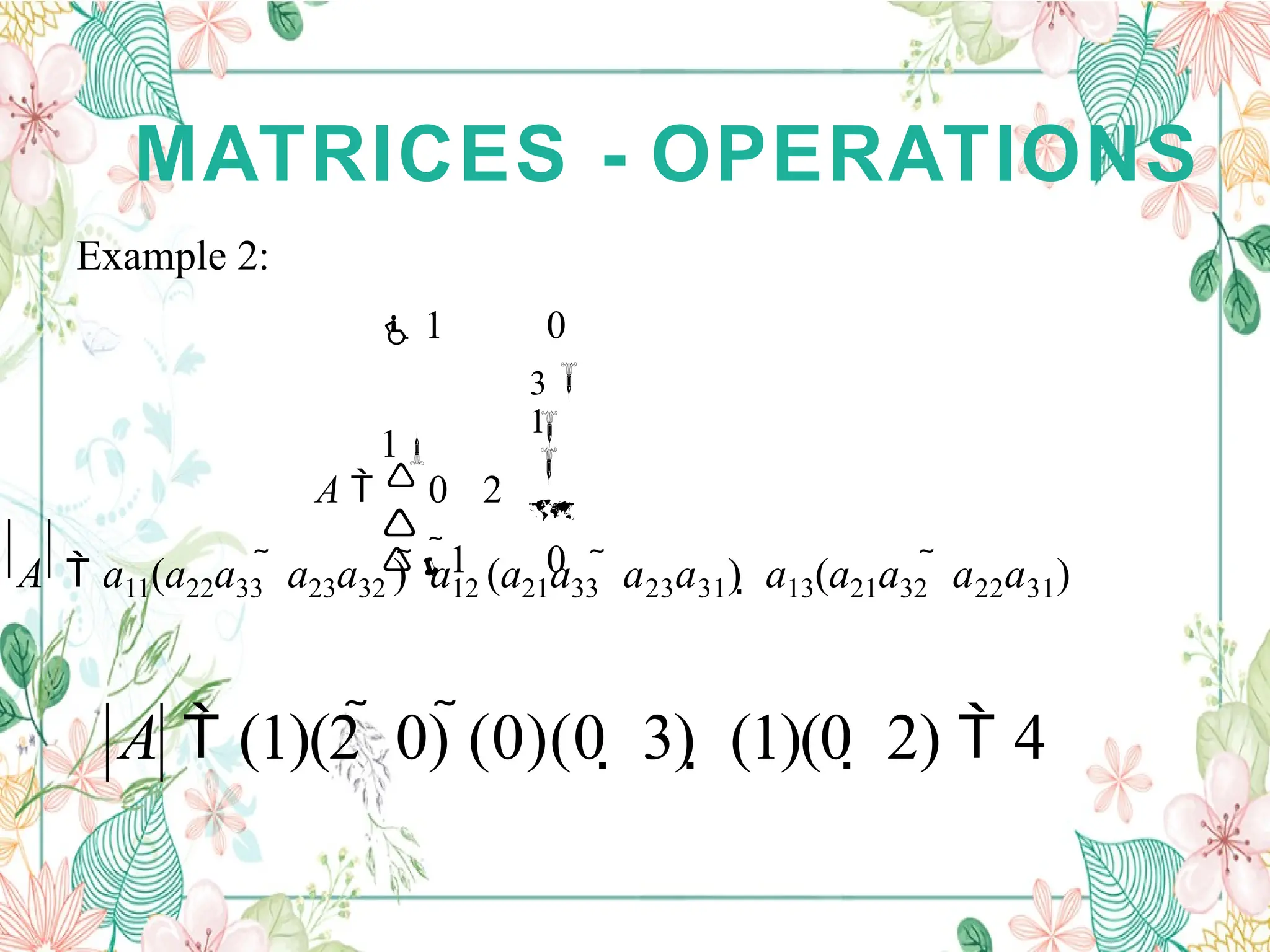
Which by substituting for the cofactors in this case is:
A a11(a22a33 a23a32 ) a12 (a21a33 a23a31) a13(a21a32 a22a31)
MATRICES - OPERATIONS
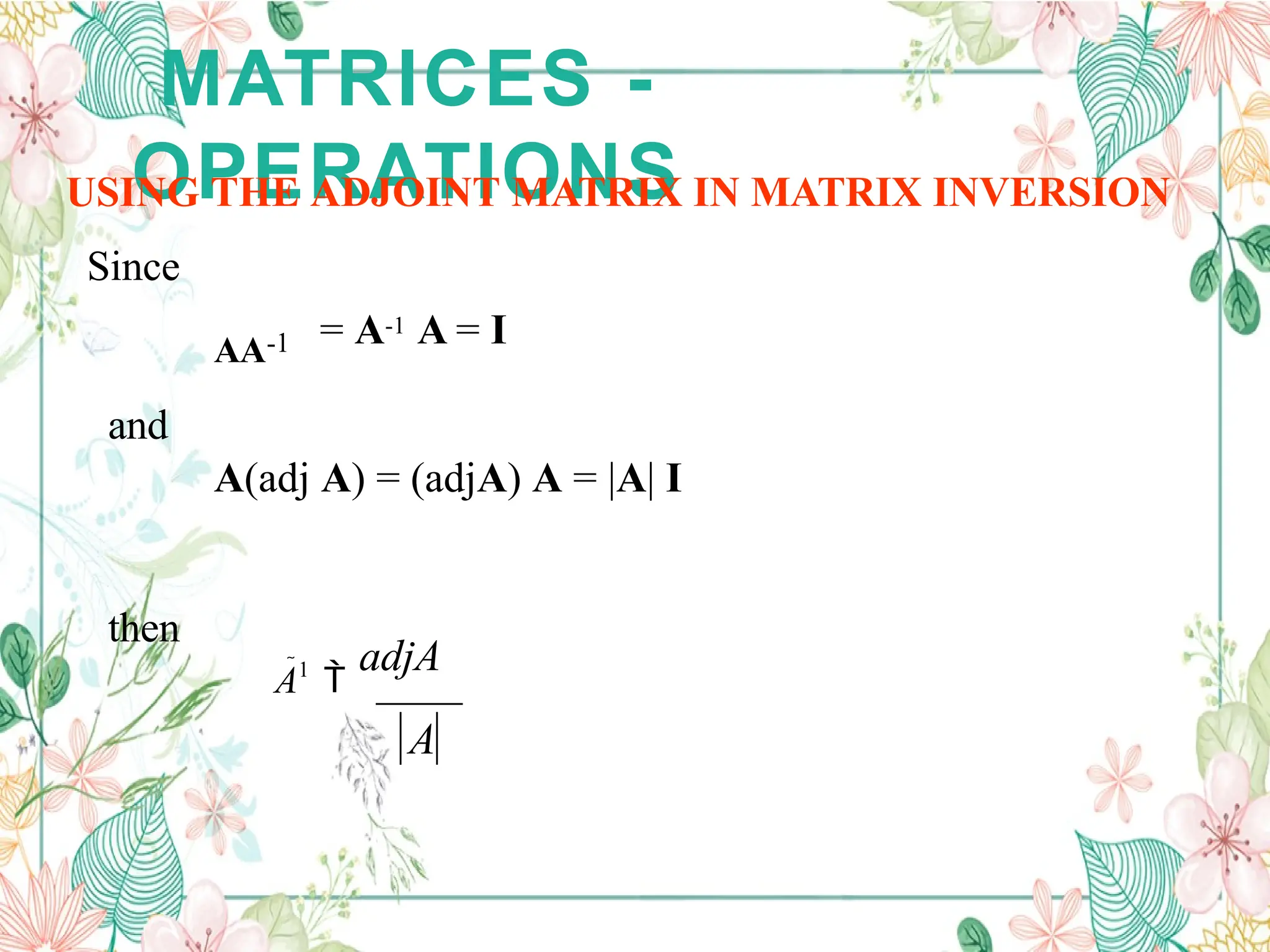
ADJOINTMATRICES
A cofactor matrix C of a matrix A is the square matrix of the same
order as A in which each element aij is replaced by its cofactor cij .
Example:
4
2
3
A
1
1
4
3
C 2
If
The cofactor C of A
is
38.
MATRICES -
OPERATIONS
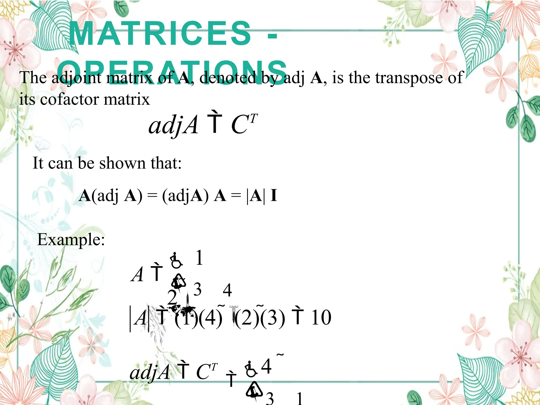
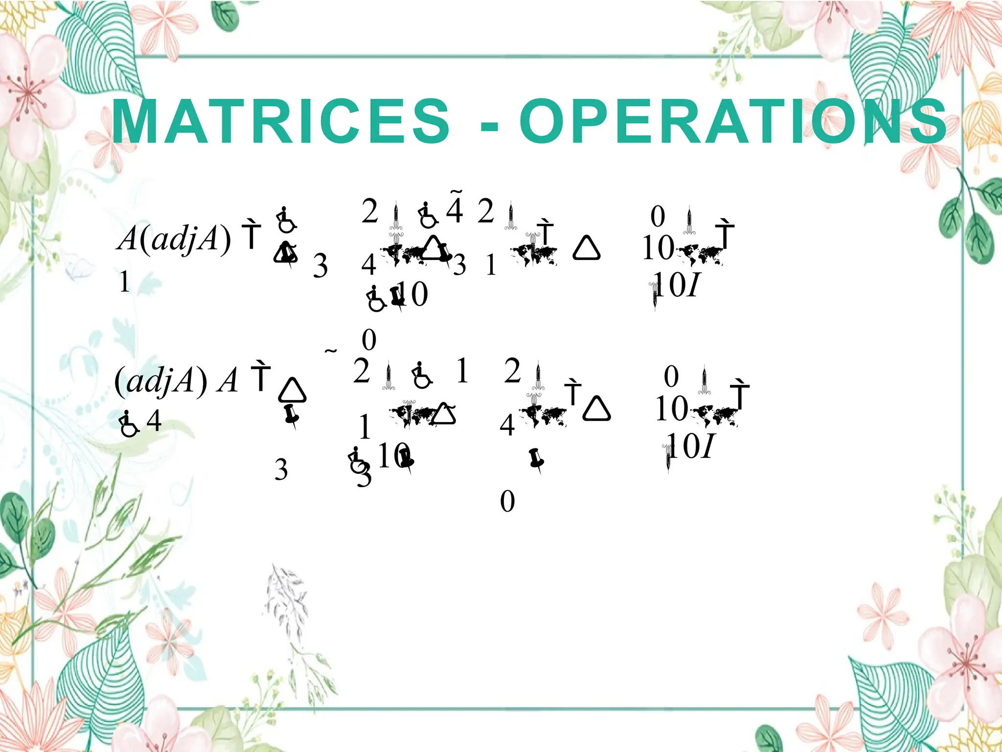
The adjointmatrix of A, denoted by adj A, is the transpose of
its cofactor matrix
adjA CT
It can be shown that:
A(adj A) = (adjA) A = |A| I
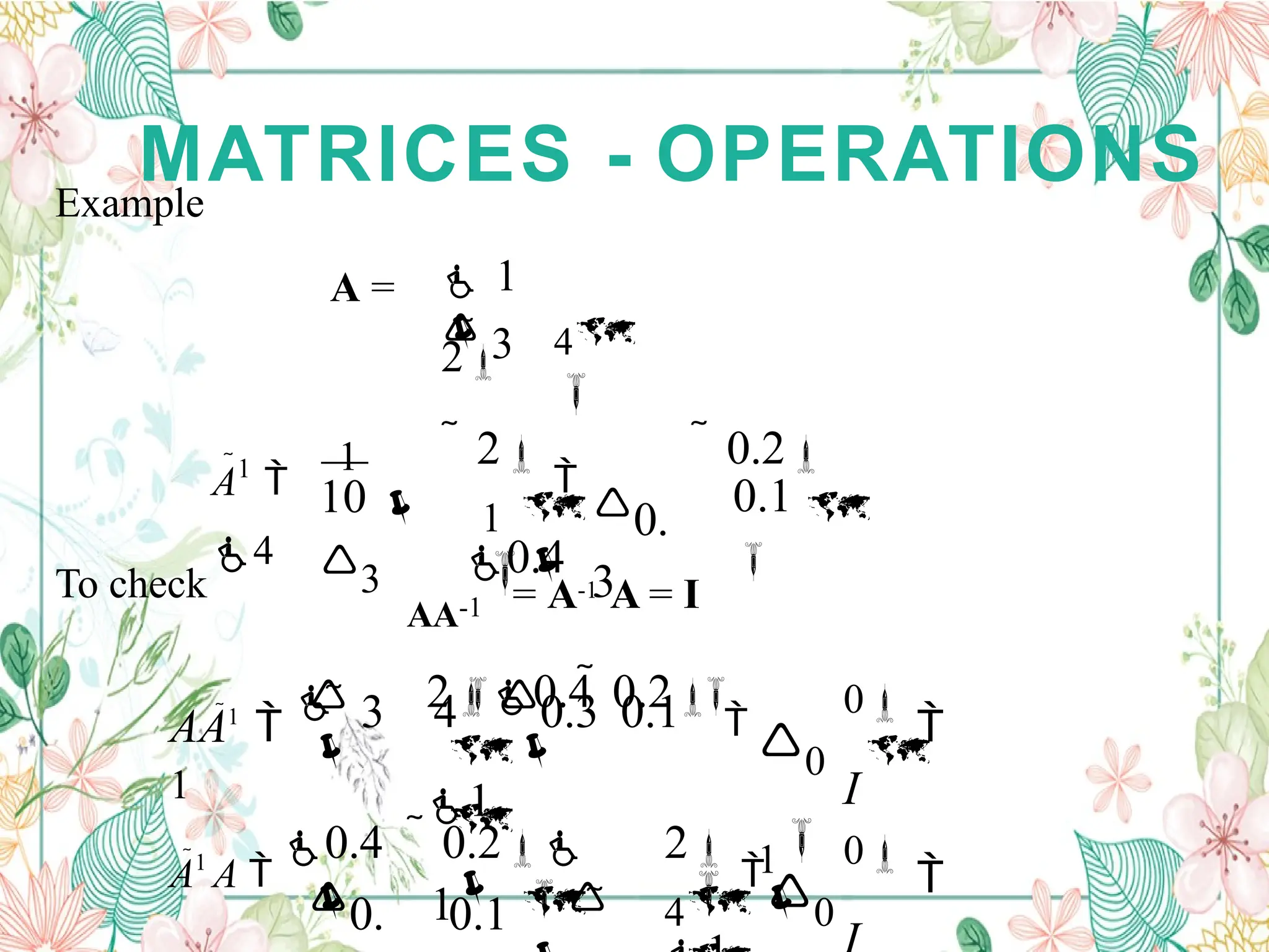
Example:
4
adjA CT
A (1)(4) (2)(3) 10
4
1
2
A 3
MATRICES -
OPERATIONS
The resultcan be checked using
AA-1 = A-1 A = I
The determinant of a matrix must not be zero for the inverse
to exist as there will not be a solution
Nonsingular matrices have non-zero determinants
Singular matrices have zero determinants
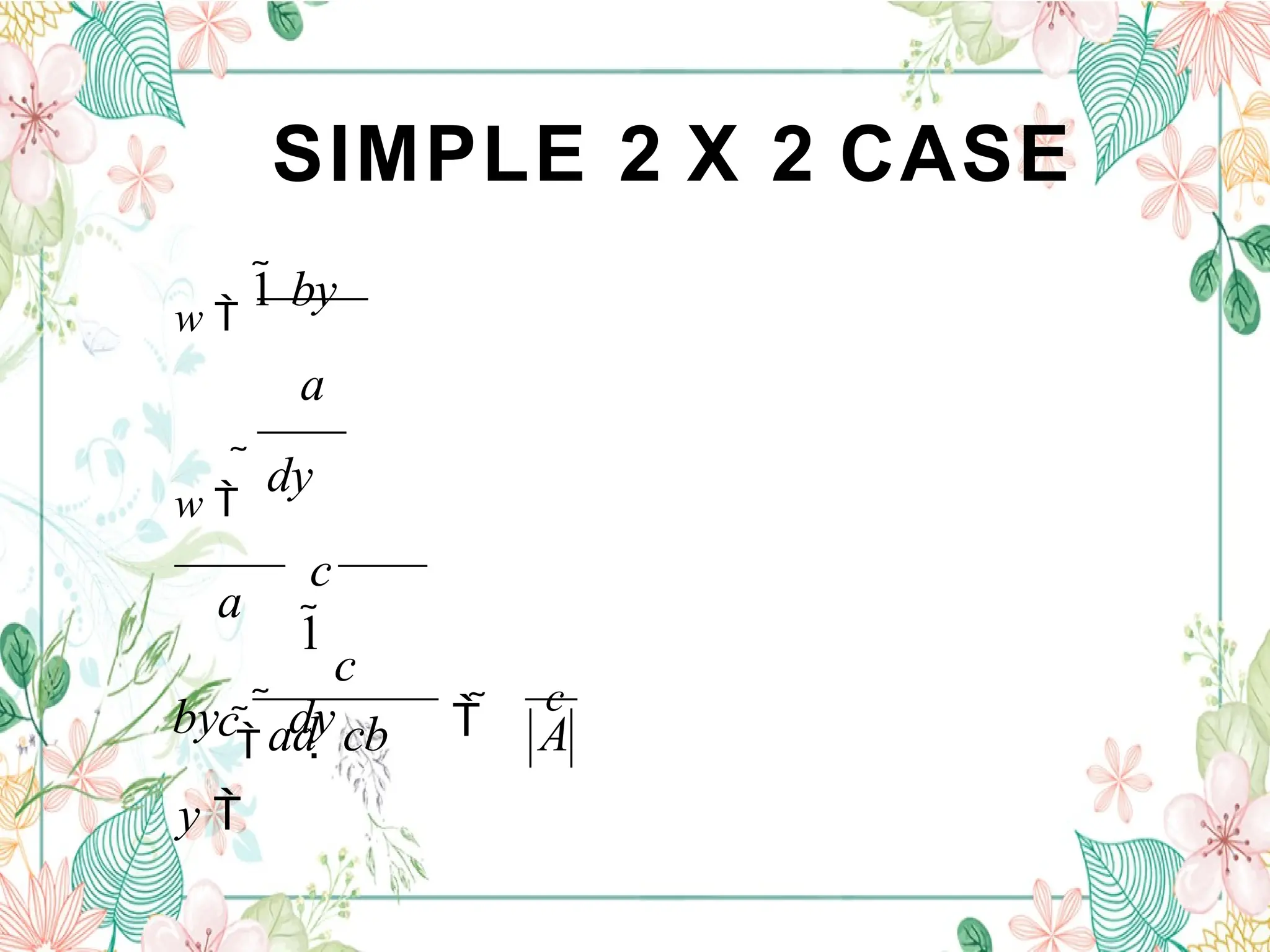
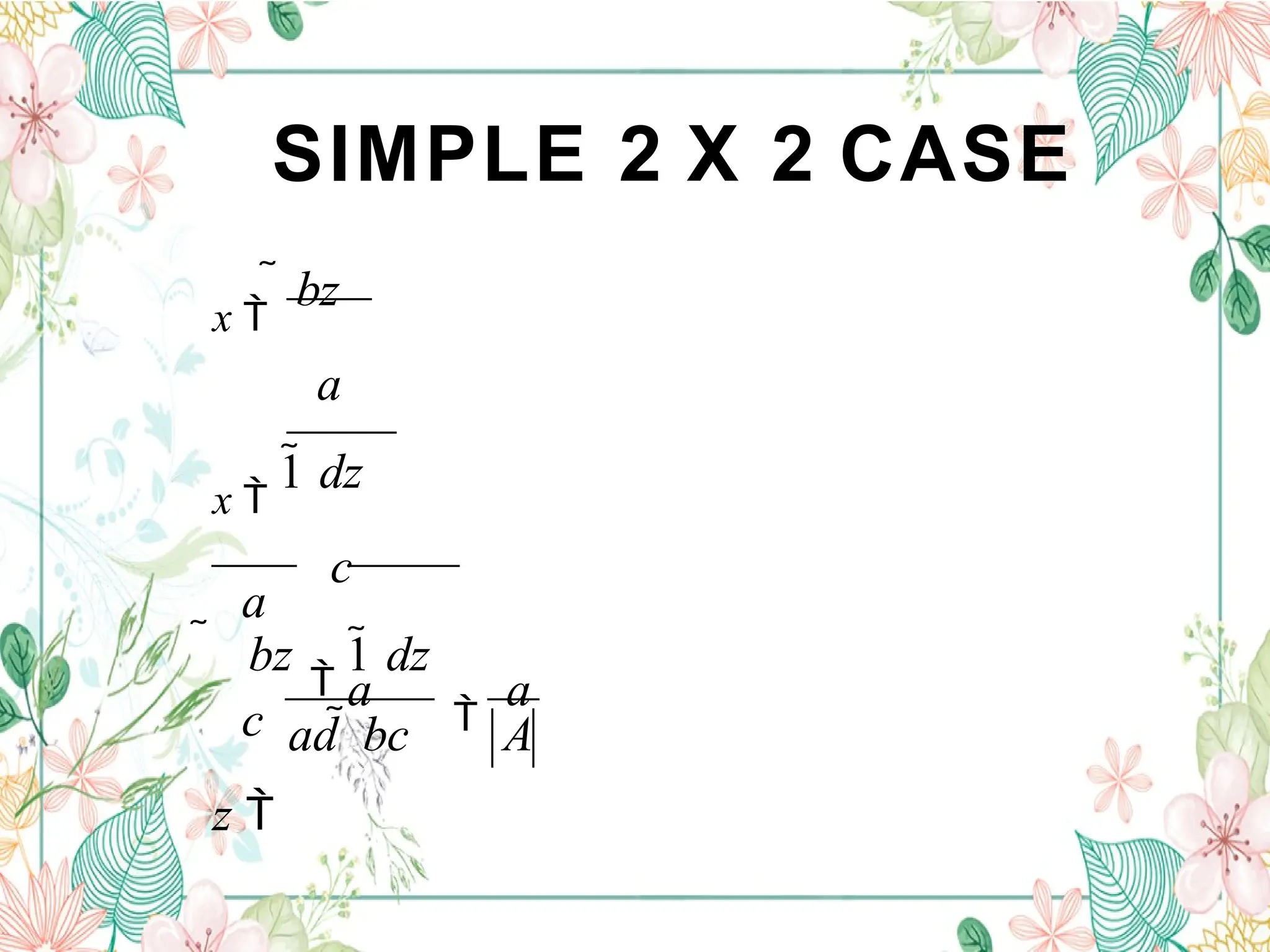
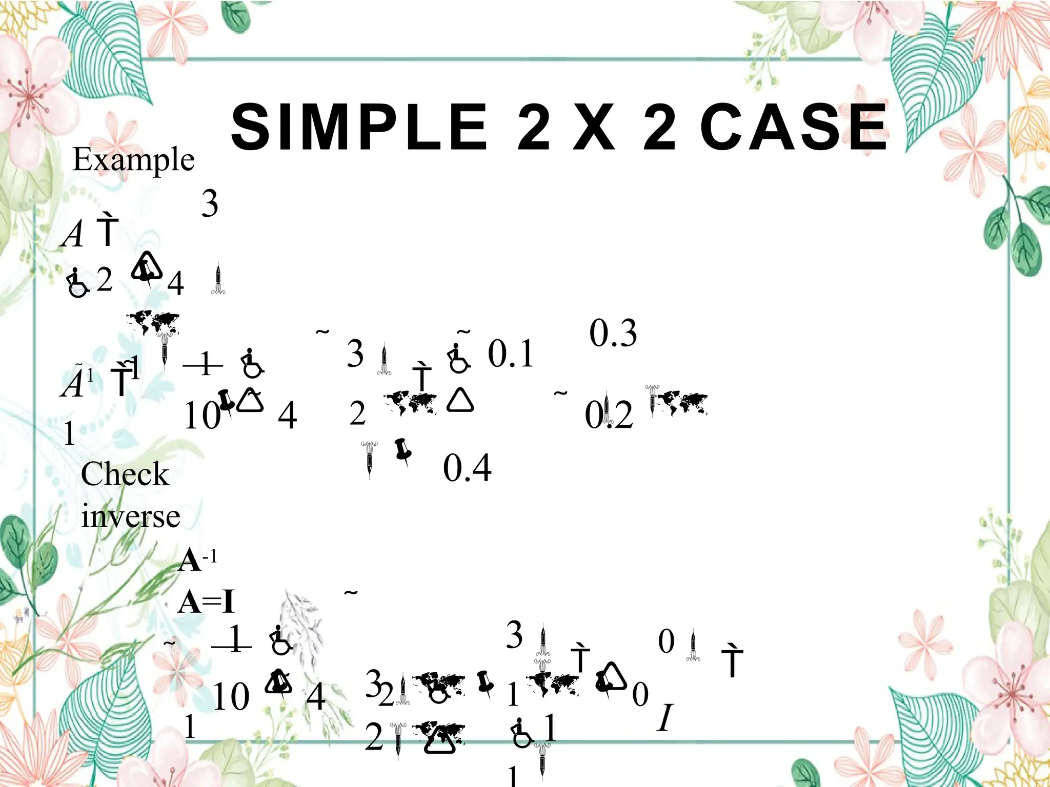
SIMPLE 2
X 2CASE
Let
c d
a b
A
and
y
z
w
x
A1
Since it is known that
A A-1 = I
then
z 0
1
c d
y
bwx
1
0
a
47.
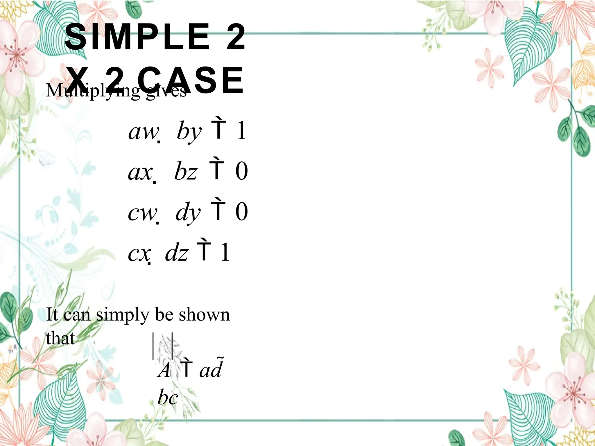
SIMPLE 2
X 2CASE
Multiplying gives
aw by 1
ax bz 0
cw dy 0
cx dz 1
It can simply be shown
that
A ad
bc
48.
SIMPLE 2 X2 CASE
thus
y
1 aw
b
y
cw
d
1
aw
cw
d
d
da bc A
b
d
w
49.
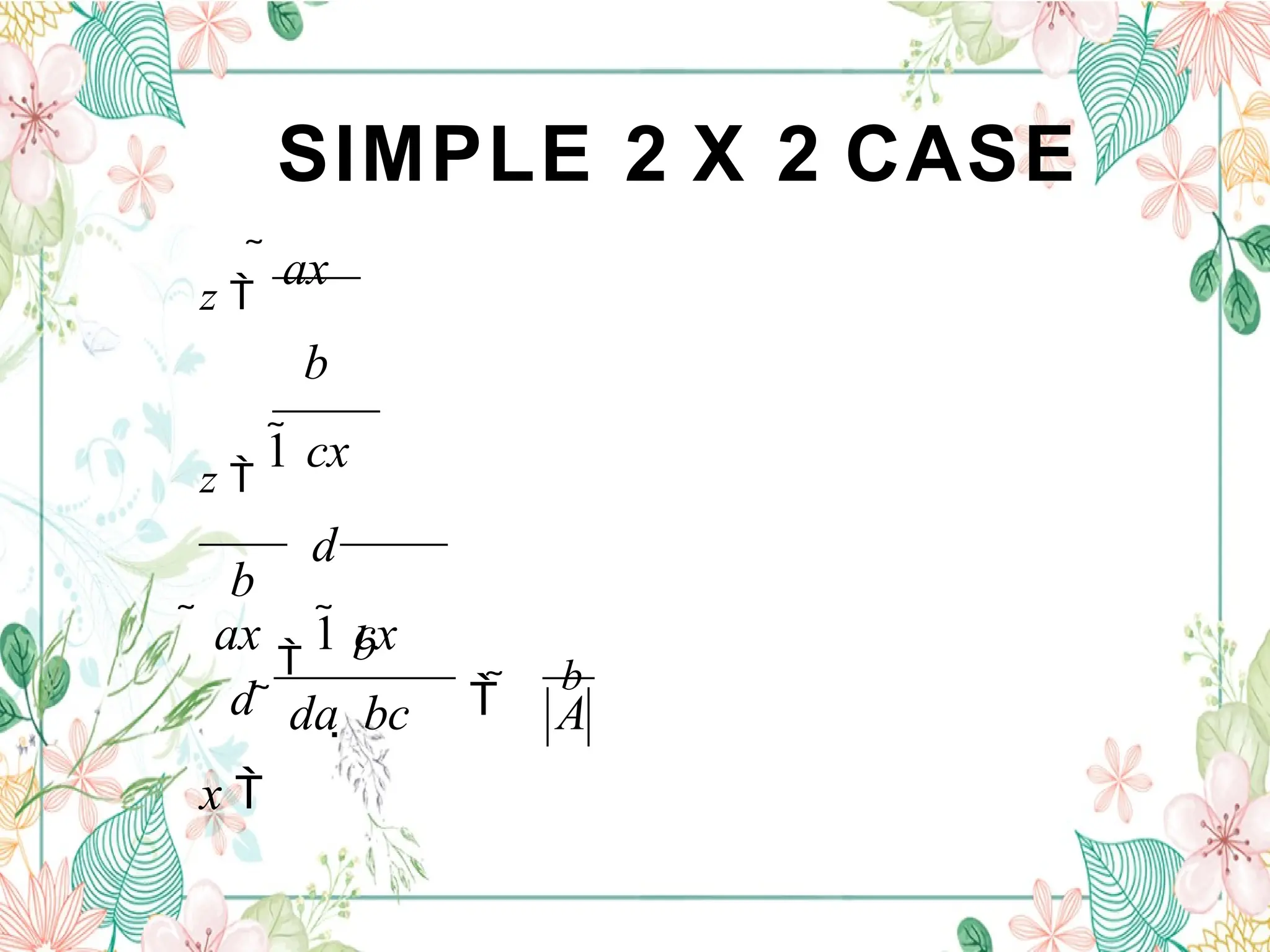
SIMPLE 2 X2 CASE
A
b
b
da bc
b
d
x
z
ax
b
z
1 cx
d
ax
1 cx
50.
SIMPLE 2 X2 CASE
A
c
c
ad cb
a
c
y
w
1 by
a
w
dy
c
1
by
dy
51.
SIMPLE 2 X2 CASE
a
a
ad bc A
a
c
z
x
bz
a
x
1 dz
c
bz
1 dz
52.
SIMPLE 2 X2 CASE
So that for a 2 x 2 matrix the inverse can be constructed
in a simple fashion as
a
b
a
A
c
1
d
A
A
c
d b
A
A
•Exchange elements of main diagonal
•Change sign in elements off main diagonal
•Divide resulting matrix by the determinant
y z
w
x
A
1
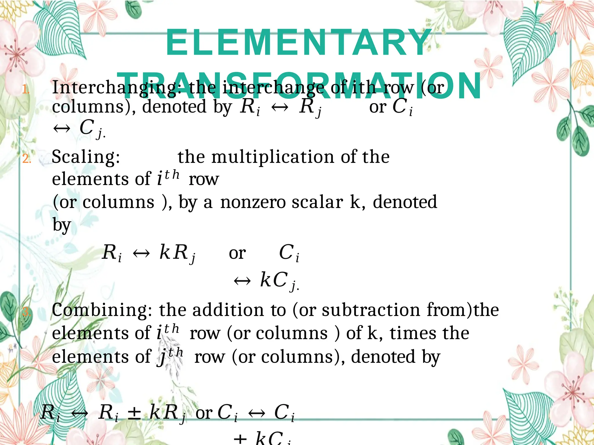
ELEMENTARY
TRANSFORMATION
1. Interchanging: theinterchange of ith row (or
columns), denoted by 𝑅𝑖 ↔ 𝑅𝑗 or 𝐶𝑖
↔ 𝐶𝑗.
2. Scaling: the multiplication of the
elements of 𝑖𝑡ℎ
row
(or columns ), by a nonzero scalar k, denoted
by
𝑅𝑖 ↔ 𝑘𝑅𝑗 or 𝐶𝑖
↔ 𝑘𝐶𝑗.
3. Combining: the addition to (or subtraction from)the
elements of 𝑖𝑡ℎ row (or columns ) of k, times the
elements of 𝑗𝑡ℎ row (or columns), denoted by
𝑅𝑖 ↔ 𝑅𝑖 ± 𝑘𝑅𝑗 or 𝐶𝑖 ↔ 𝐶𝑖
56.
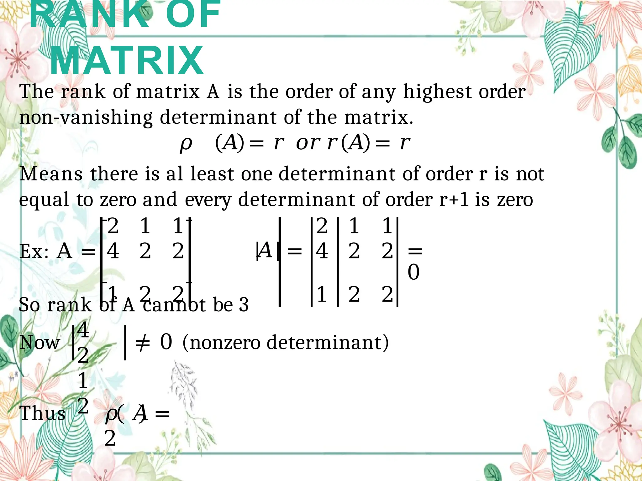
RANK OF
MATRIX
2 11 2 1 1
4 2 2 𝐴 = 4 2 2 =
0
1 2 2 1 2 2
The rank of matrix A is the order of any highest order
non-vanishing determinant of the matrix.
𝜌 𝐴 = 𝑟 𝑜𝑟 𝑟 𝐴 = 𝑟
Means there is al least one determinant of order r is not
equal to zero and every determinant of order r+1 is zero
Ex: A =
So rank of A cannot be 3
Now
4
2
1
2
≠ 0 (nonzero determinant)
Thus 𝜌 𝐴 =
2
57.
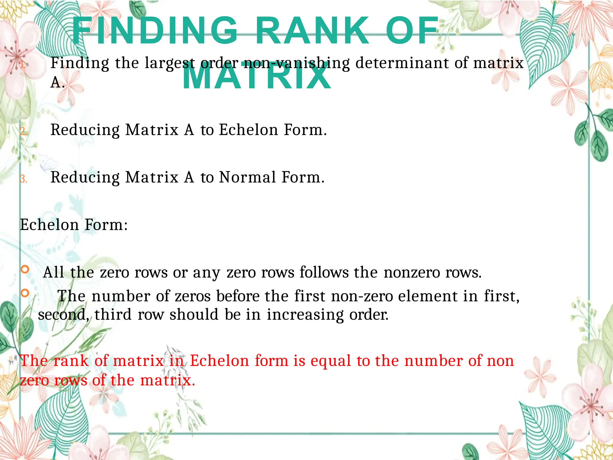
FINDING RANK OF
MATRIX
1.Finding the largest order non-vanishing determinant of matrix
A.
2. Reducing Matrix A to Echelon Form.
3. Reducing Matrix A to Normal Form.
Echelon Form:
All the zero rows or any zero rows follows the nonzero rows.
The number of zeros before the first non-zero element in first,
second, third row should be in increasing order.
The rank of matrix in Echelon form is equal to the number of non
zero rows of the matrix.
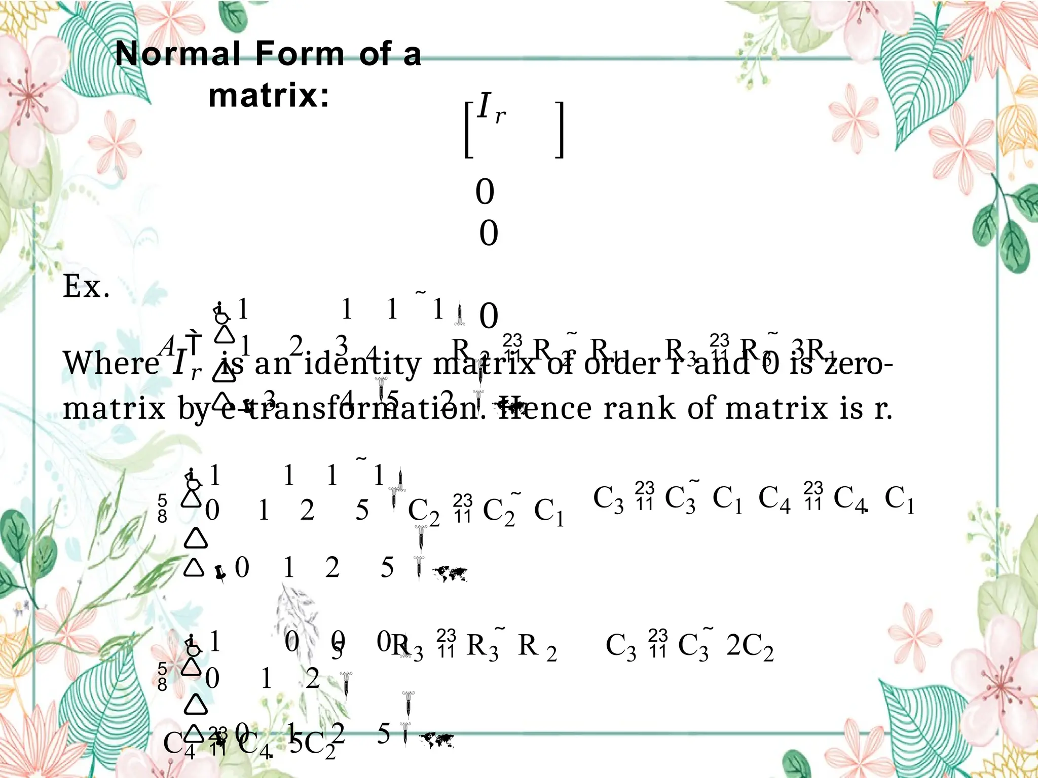
Normal Form ofa
matrix: 𝐼𝑟
0
0
0
Where 𝐼𝑟 is an identity matrix of order r and 0 is zero-
matrix by e-transformation. Hence rank of matrix is r.
Ex.
C4 C4 5C2
C3 C3 2C2
R3 R3 R 2
C3 C3 C1 C4 C4 C1
R3 R3 3R1
5
R 2 R 2 R1
4
1 1 1 1
A 1 2 3
3 4 5 2
1 1 1 1
0 1 2 5 C2 C2 C1
0 1 2 5
1 0 0 0
0 1 2
0 1 2 5
60.
( A)
2
0
10
0
0
0 1 0
0 0 0
0
I2
Hence
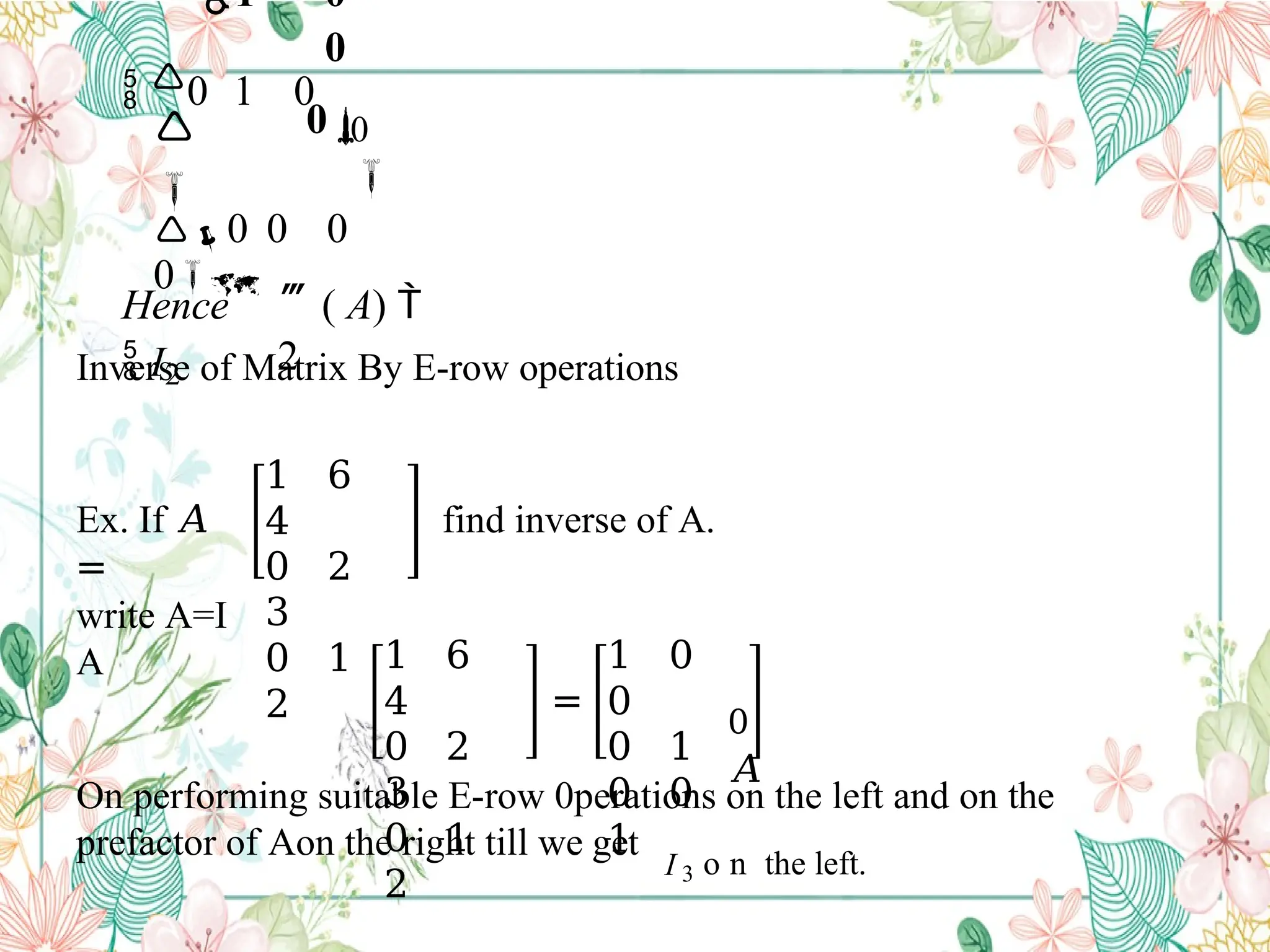
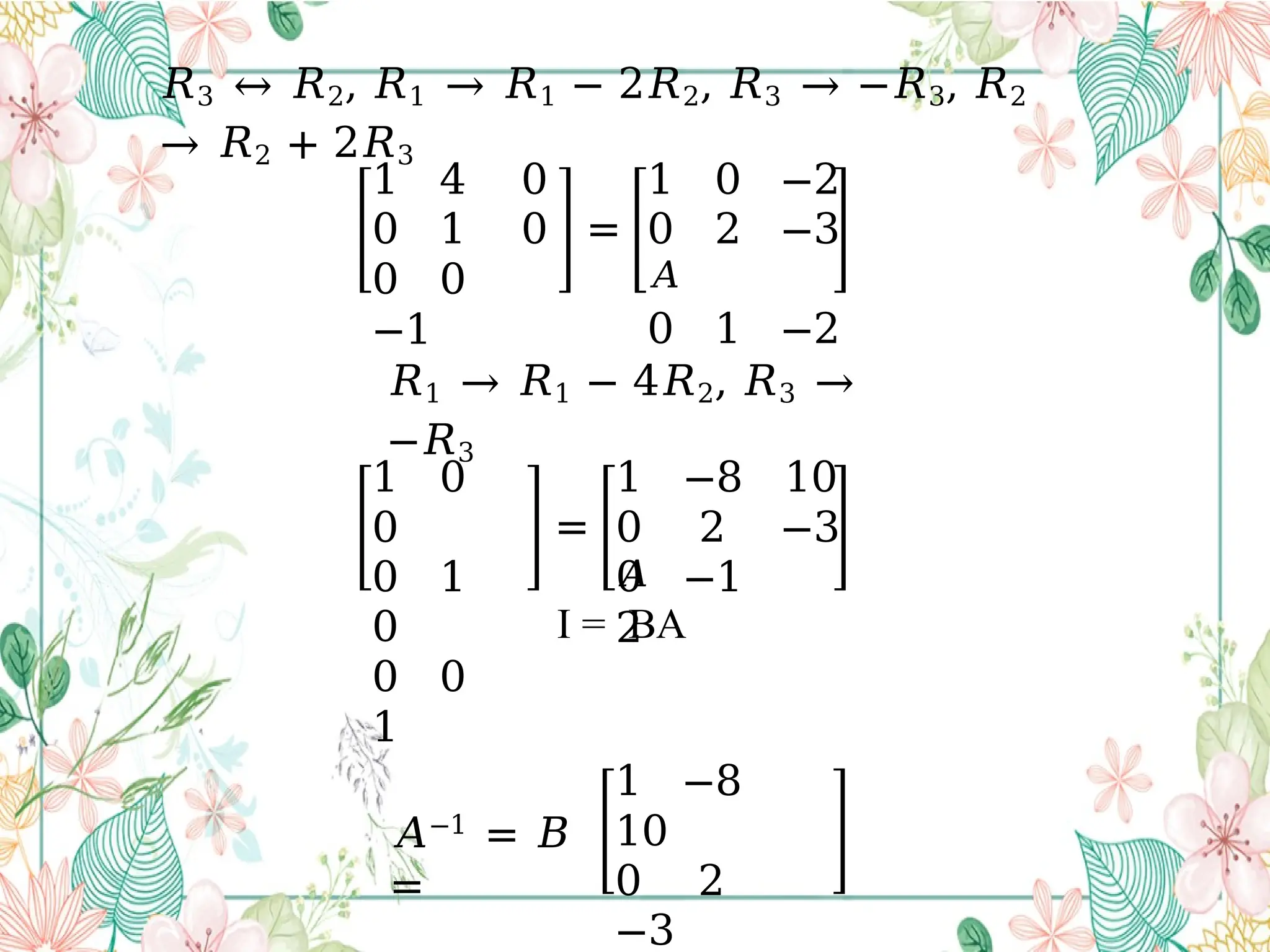
Inverse of Matrix By E-row operations
Ex. If 𝐴
=
1 6
4
0 2
3
0 1
2
find inverse of A.
write A=I
A 1 6
4
0 2
3
0 1
2
=
1 0
0
0 1
0 0
1
0
𝐴
On performing suitable E-row 0perations on the left and on the
prefactor of Aon the right till we get
I 3 o n the left.
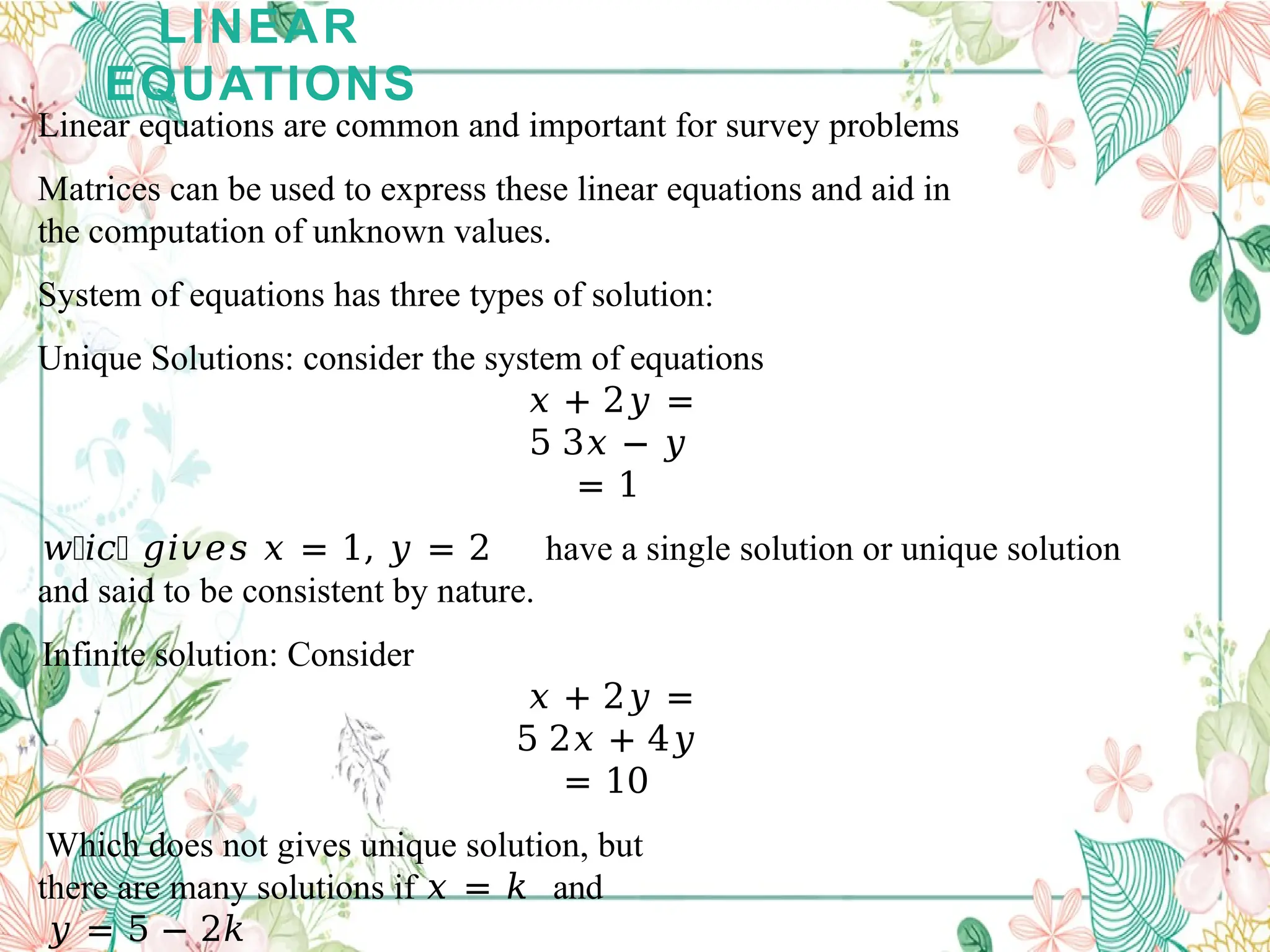
LINEAR
EQUATIONS
Linear equations arecommon and important for survey problems
Matrices can be used to express these linear equations and aid in
the computation of unknown values.
System of equations has three types of solution:
Unique Solutions: consider the system of equations
𝑥 + 2𝑦 =
5 3𝑥 − 𝑦
= 1
𝑤𝑖𝑐 𝑔𝑖𝑣𝑒𝑠 𝑥 = 1, 𝑦 = 2 have a single solution or unique solution
and said to be consistent by nature.
Infinite solution: Consider
𝑥 + 2𝑦 =
5 2𝑥 + 4𝑦
= 10
Which does not gives unique solution, but
there are many solutions if 𝑥 = 𝑘 and
𝑦 = 5 − 2𝑘
64.
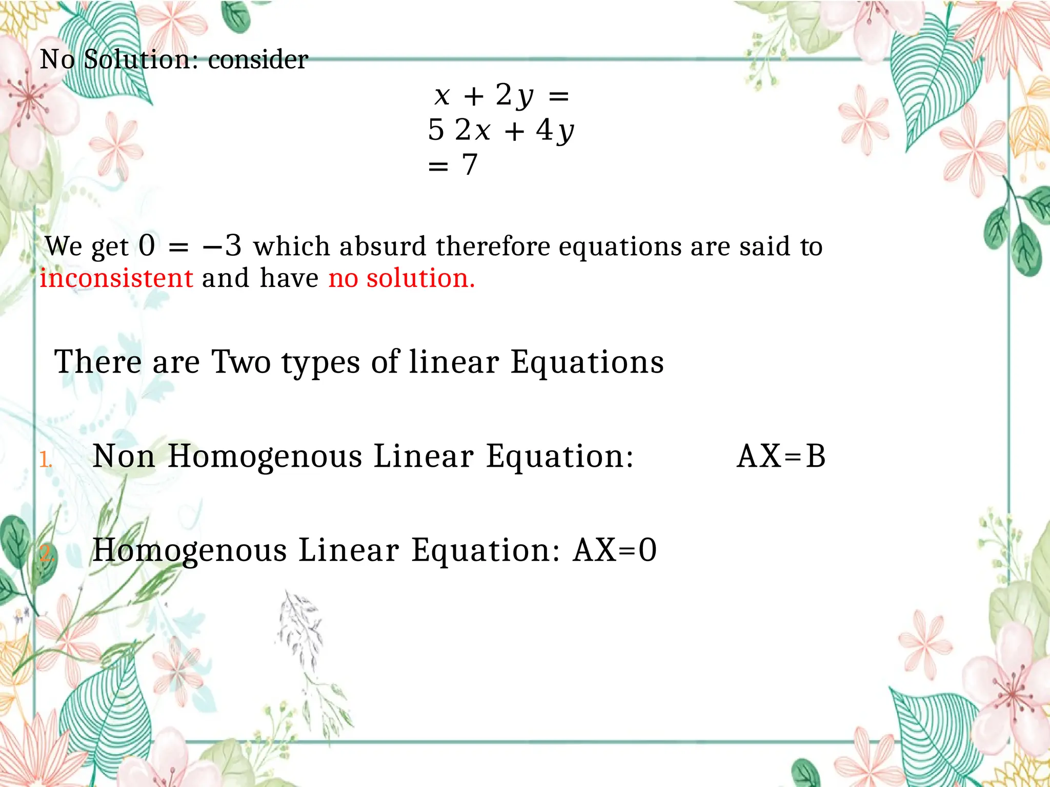
No Solution: consider
𝑥+ 2𝑦 =
5 2𝑥 + 4𝑦
= 7
We get 0 = −3 which absurd therefore equations are said to
inconsistent and have no solution.
There are Two types of linear Equations
1. Non Homogenous Linear Equation: AX=B
2. Homogenous Linear Equation: AX=0
65.
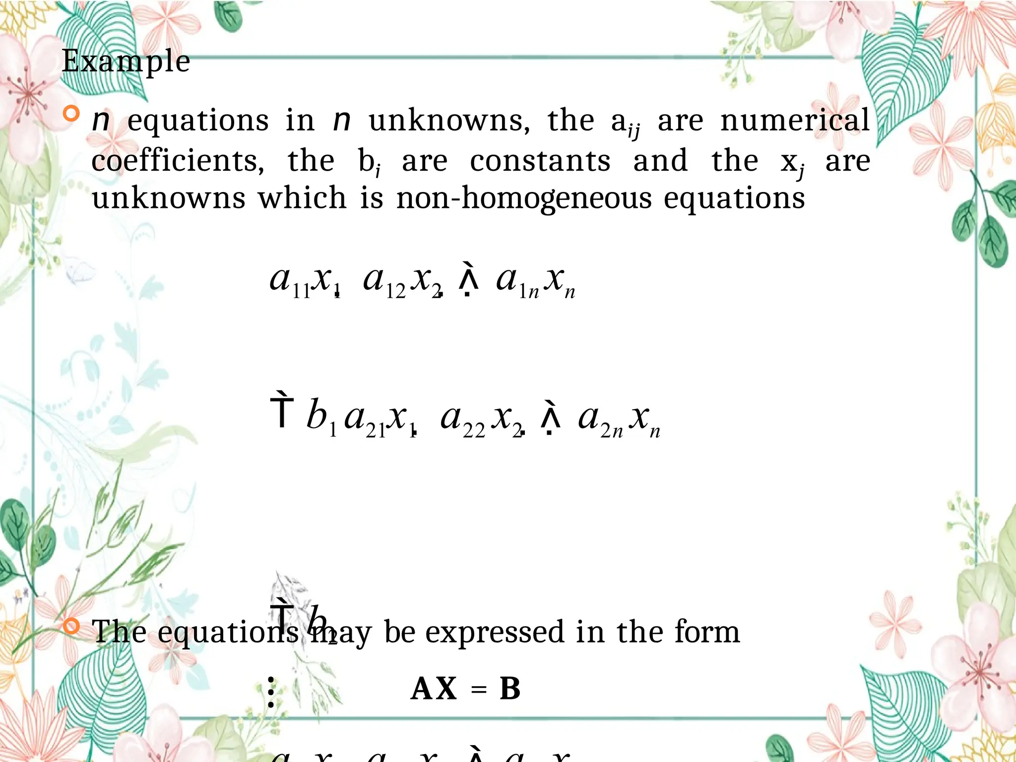
Example
n equationsin n unknowns, the aij are numerical
coefficients, the bi are constants and the xj are
unknowns which is non-homogeneous equations
a11x1 a12 x2 a1n xn
b1 a21x1 a22 x2 a2n xn
b2
⁝
The equations may be expressed in the form
AX = B
66.
x
x1
ann
xn
a
a1n
a1
1
a
⁝
a
A
21 22
⁝ ⁝
an1
an1
a12
2n
, X
2
,and B
⁝
bn
n x
1
b
b
⁝
2
1
n x n n x 1
Number of unknowns = number of equations = n
Augmented Matrix: The matrix composed of mn elements
of
coefficient matrix A plus one addition column whose
elements are constant 𝑏𝑖 is called augmented matrix of the
system and denoted [A, B]
b
a
[ A, B]
b2
a12 ...
a1n b1
a22 ...
a2n
a11
a2
1
67.
Solution Of nonHomogenous Equation:
If There are n Equations in n Variables
a) If 𝜌 𝐴 = 𝜌 𝐴, 𝐵 = 𝑟 = 𝑛(number of variables), the system
will have Unique solution.
b)
If 𝜌 𝐴
= 𝜌
𝐴, 𝐵
= 𝑟 < 𝑛, the system will have
infinite
solution.
c)
If 𝜌 𝐴
≠ 𝜌
𝐴, 𝐵
the system will have no solution.
Example: solve the system of equation
2𝑥 + 𝑦 − 2𝑧
= 2
𝑥 + 𝑦 + 𝑧
= 4 3𝑥 − 𝑦
+ 𝑧 = 2
𝑥 + 2𝑦 + 2𝑧
= 7
Here
AX=B
7
2
4
2
2
1
1
1
1
z
y
2 1 2
x
1
Example: Solve theequations such that equations have (i) no Solution
(ii) a
Unique solution (iii) a Infinite solution
𝑥 + 𝑦 + 𝑧 = 6
𝑥 + 2𝑦 + 3𝑧 =
10
𝑥 + 2𝑦 + 𝑎𝑧 =
𝑏
Here
1 1
1
1 2
3
1 2
𝑎
�
�
�
�
�
�
=
6
1
0
𝑏
Then augmented matrix
b
1 1 1 ...
6
0 1 2 ...
4
R2 R2 R1, R3 R3 R2
1 1 1 ... 6
2 3 ...
10
1 2 a ...
b
[ A, B]
1
71.
Case I: when𝑎 = 3, 𝑏 ≠ 10 we get
𝜌 𝐴 = 2 𝜌 𝐴, 𝐵 = 3
Thus system is inconsistent and have no solution.
Case II: when 𝑎 = 3, 𝑏 = 10 we get
𝜌 𝐴 = 𝜌 𝐴, 𝐵 = 2 < 3 𝑁𝑜. 𝑜𝑓 𝑣𝑎𝑟𝑖𝑎𝑏𝑙𝑒𝑠
Thus system is consistent and infinite solution.
Case III: when 𝑎 ≠ 3 we get
𝜌 𝐴 = 𝜌 𝐴, 𝐵 = 3(𝑁𝑜. 𝑜𝑓 𝑣𝑎𝑟𝑖𝑎𝑏𝑙𝑒𝑠)
Thus system is consistent and have unique solution.
72.
HOMOGENOUS
LINEAR
EQUATION
when the systemhas n Equations in n variables
The equation AX=0 will always have unique solution if rank of A is
always equal to number of variables, but it is zero solution also Known as
Trivial solution. In this case A is non singular matrix i.e. 𝐴 ≠
0.
When rank of matrix A is r less than number of variables then there will be
infinite solutions
In this case 𝐴 = 0 and we have non zero solution called non trivial
solution.
Example: Solve
𝑥 − 𝑦 + 𝑧 = 0
𝑥 + 2𝑦 − 𝑧 =
0 2𝑥 + 𝑦 −
3𝑧 = 0
matrix equation becomes
1 −1 1
1 2
−1
2 1
−3
�
�
�
�
�
=
0
0
0
AX=0
73.
The Coefficient matrix
1−1 1
𝐴 = 1 2 −1
2 1 −3
[𝑅2 → 𝑅2 − 𝑅1, 𝑅3 → 𝑅3 − 2 𝑅1]
and then
[𝑅3 → 𝑅3 − 𝑅2]
𝐴
=
1 −1 1
0 3
−2
0 0 3
This is Echelon form and rank of A =3 (No. of variables). Therfore
zero solution is the only solution.
Now matrix equation
𝑥 − 𝑦 + 𝑧 = 0
3𝑦 − 2𝑧 = 0
3𝑧 = 0
Which gives x=0,y=0 and z=0.
74.
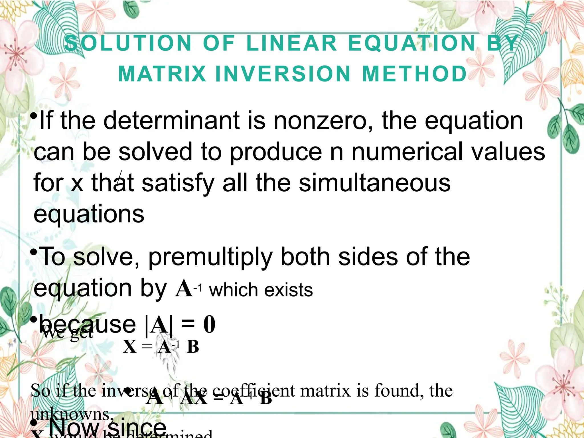
SOLUTION OF LINEAREQUATION BY
MATRIX INVERSION METHOD
•If the determinant is nonzero, the equation
can be solved to produce n numerical values
for x that satisfy all the simultaneous
equations
•To solve, premultiply both sides of the
equation by A-1 which exists
•because |A| = 0
• A-1 AX = A-1 B
• Now since
We get
X = A-1 B
So if the inverse of the coefficient matrix is found, the
unknowns,
75.
LINEAR
EQUATION
S
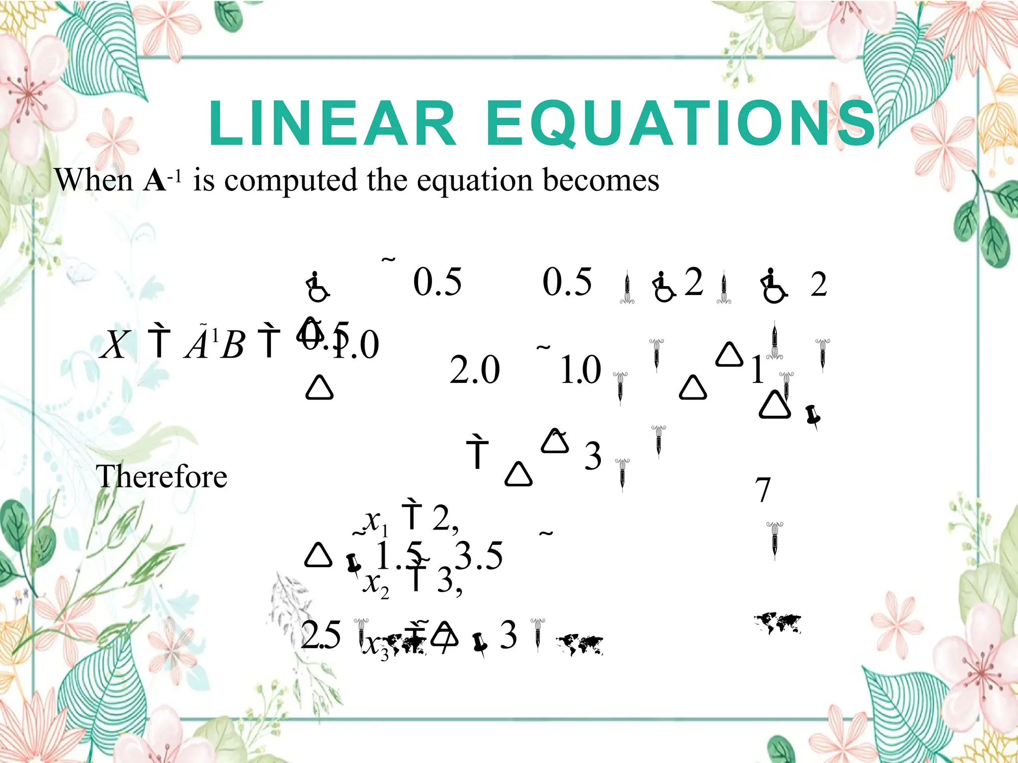
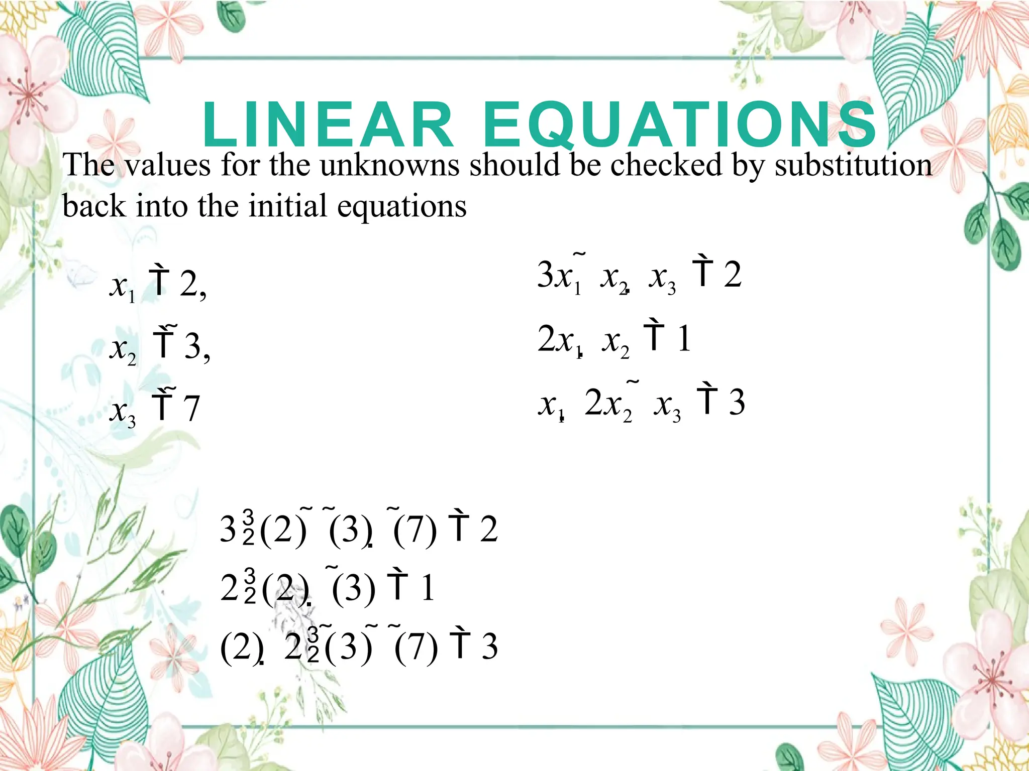
Example
3x1 x2 x3 2
2x1 x2 1
x1 2x2 x3 3
The equations can be expressed as
1
x3
3
2
0 x
1
1 x1
2
1
2
3 1
1
2

![DEFINITIO
N
A matrix is a set or group of numbers arranged in a square or
rectangular array enclosed by two brackets
Example 1:
PROPERTIES:
A specified number of rows and a specified number of columns
Two numbers (rows x columns) describe the dimensions or
size of the matrix or we say order of the matrix.
[4 2
3 0]](https://image.slidesharecdn.com/matrices-250623180042-caf30845/75/MATRICES-CSEC-MATHEMATICS-SECTION-TWO-2-2048.jpg)
![DEFINITIO
N
PROPERTIES:
A specified number of rows and a specified number of columns
Two numbers (rows × columns) describe the dimensions or size of the matrix
or we say order of the matrix.
Example 2:
- 1 x 2 matrix (1 row, 2 columns)
- 2 x 2 matrix (1 row, 2 columns)
- 2 x 4 matrix (1 row, 2 columns)
[4 2
3 0]](https://image.slidesharecdn.com/matrices-250623180042-caf30845/75/MATRICES-CSEC-MATHEMATICS-SECTION-TWO-3-2048.jpg)
![MATRICES - OPERATIONS
If A = [A] is a single element (1x1), then the determinant
is defined as the value of the element
Then |A| =det A = a11
If A is (n x n), its determinant may be defined in terms of
order (n-1) or less.](https://image.slidesharecdn.com/matrices-250623180042-caf30845/75/MATRICES-CSEC-MATHEMATICS-SECTION-TWO-26-2048.jpg)


![
x
x1
ann
xn
a
a1n
a1
1
a
⁝
a
A
21 22
⁝ ⁝
an1
an1
a12
2n
, X
2
,and B
⁝
bn
n x
1
b
b
⁝
2
1
n x n n x 1
Number of unknowns = number of equations = n
Augmented Matrix: The matrix composed of mn elements
of
coefficient matrix A plus one addition column whose
elements are constant 𝑏𝑖 is called augmented matrix of the
system and denoted [A, B]
b
a
[ A, B]
b2
a12 ...
a1n b1
a22 ...
a2n
a11
a2
1](https://image.slidesharecdn.com/matrices-250623180042-caf30845/75/MATRICES-CSEC-MATHEMATICS-SECTION-TWO-66-2048.jpg)
![Augmented
Matrix2
[R2 R 4 ] [R3 R3 4R 2, R 4 R 4 R 2 ]
[R 4
1
R 4, R3
1
R3]
3 2
[R4 R 4 R3]
[R2 R 2 2R1, R3 R3 3R1
2
2
4
3
1
7
R 4 R 4 R1]
1
2
1 1 ...
1 2 ...
1 1 ...
2 2 ...
R1 R 2
7
1 2 ...
1 1 ...
1 1 ...
2 2 ...
3
1
2
4
1
2
[ A, B]
](https://image.slidesharecdn.com/matrices-250623180042-caf30845/75/MATRICES-CSEC-MATHEMATICS-SECTION-TWO-68-2048.jpg)
![Which is Echelon form of Matrix [A,B]
𝜌 𝐴 = 𝜌 𝐴, 𝐵therefore equations are consistent.
Now 𝜌 𝐴 = 𝜌 𝐴, 𝐵 = 3 = 𝑛(number of
variables), the system will have
Unique solution.
𝑥 + 𝑦 + 𝑧
= 4
𝑦 + 𝑧 = 3
𝑧 = 1
0
3
0 1 1 ...
0 0 1 ...
1
0 0 0 ...
1 1 1
...
4
0
1
3
4
0
0
1
0
1 1
1
0 0
0
1
z
y
1
x](https://image.slidesharecdn.com/matrices-250623180042-caf30845/75/MATRICES-CSEC-MATHEMATICS-SECTION-TWO-69-2048.jpg)
![Example: Solve the equations such that equations have (i) no Solution
(ii) a
Unique solution (iii) a Infinite solution
𝑥 + 𝑦 + 𝑧 = 6
𝑥 + 2𝑦 + 3𝑧 =
10
𝑥 + 2𝑦 + 𝑎𝑧 =
𝑏
Here
1 1
1
1 2
3
1 2
𝑎
�
�
�
�
�
�
=
6
1
0
𝑏
Then augmented matrix
b
1 1 1 ...
6
0 1 2 ...
4
R2 R2 R1, R3 R3 R2
1 1 1 ... 6
2 3 ...
10
1 2 a ...
b
[ A, B]
1](https://image.slidesharecdn.com/matrices-250623180042-caf30845/75/MATRICES-CSEC-MATHEMATICS-SECTION-TWO-70-2048.jpg)
![The Coefficient matrix
1 −1 1
𝐴 = 1 2 −1
2 1 −3
[𝑅2 → 𝑅2 − 𝑅1, 𝑅3 → 𝑅3 − 2 𝑅1]
and then
[𝑅3 → 𝑅3 − 𝑅2]
𝐴
=
1 −1 1
0 3
−2
0 0 3
This is Echelon form and rank of A =3 (No. of variables). Therfore
zero solution is the only solution.
Now matrix equation
𝑥 − 𝑦 + 𝑧 = 0
3𝑦 − 2𝑧 = 0
3𝑧 = 0
Which gives x=0,y=0 and z=0.](https://image.slidesharecdn.com/matrices-250623180042-caf30845/75/MATRICES-CSEC-MATHEMATICS-SECTION-TWO-73-2048.jpg)