Downloaded 367 times
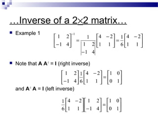
![…Matrix operations: transpose…
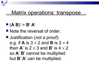
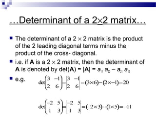
If B = AT
, then bij = aji
i.e. the transpose of an m × n matrix is an n × m matrix with the rows
and columns swapped.
e.g.
−
−−
=
−
−
−
4641
1230
3925
413
629
432
105
T
[ ]3925
3
9
2
5
−−=
−
−
T](https://image.slidesharecdn.com/random-140505135713-phpapp01/85/systems-of-linear-equations-matrices-12-320.jpg)
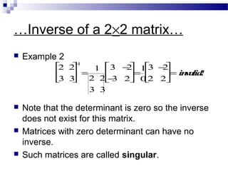
![Special matrices: row and column
A 1 × n matrix is called a row matrix.
e.g.
An m × 1 matrix is called a column matrix.
e.g.
1 columns→
3 rows
↓
3
−1
5
6 columns→
1 rows
↓
2 1 1 −2 1 −5[ ]](https://image.slidesharecdn.com/random-140505135713-phpapp01/85/systems-of-linear-equations-matrices-14-320.jpg)
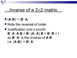
![Special matrices: square
An n × n matrix is called a square matrix.
i.e. a square matrix has the same number
of rows and columns.
e.g.
[ ]
−−
−−
−−
−
4705
7350
0523
5031
211
010
210
21
32
1](https://image.slidesharecdn.com/random-140505135713-phpapp01/85/systems-of-linear-equations-matrices-15-320.jpg)
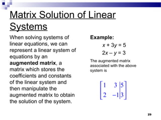
![Special matrices: diagonal
A square matrix is diagonal if non-zero elements only occur on the leading diagonal.
i.e. aij = 0 for i ≠ j
e.g.
Premultiplying a matrix by a diagonal matrix scales each row by the diagonal
element.
Postmultiplying a matrix by a diagonal matrix scales each column by the diagonal
element.
[ ]
−
4000
0300
0020
0001
200
010
000
20
02
1](https://image.slidesharecdn.com/random-140505135713-phpapp01/85/systems-of-linear-equations-matrices-16-320.jpg)
![Special matrices: null
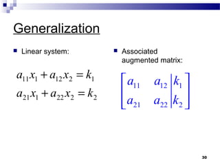
The null matrix, 0, behaves like 0 in arithmetic addition
and subtraction.
Null matrices can be of any order and have all of their
elements zero.
[ ]
[ ]
=
=
=
=
0000
0000
0000
0000
00
00
00
00
00
000
0
00
0
0](https://image.slidesharecdn.com/random-140505135713-phpapp01/85/systems-of-linear-equations-matrices-18-320.jpg)
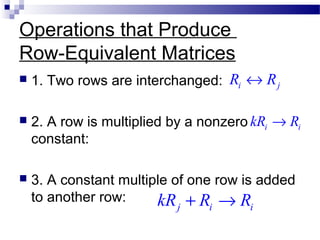
![Special matrices: identity…
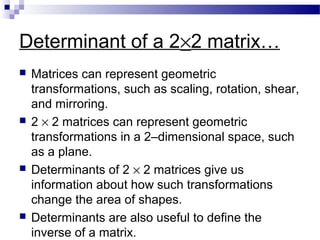
The identity matrix, I, behaves like 1 in arithmetic multiplication.
Identity matrices are diagonal. They have 1s on the diagonal and 0s
elsewhere.
e.g.
In the world of the matrix the identity truly is ‘the one’.
[ ]
=
=
==
1000
0100
0010
0001
100
010
001
10
01
1
II
II](https://image.slidesharecdn.com/random-140505135713-phpapp01/85/systems-of-linear-equations-matrices-19-320.jpg)


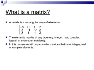
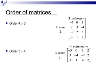
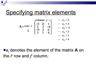
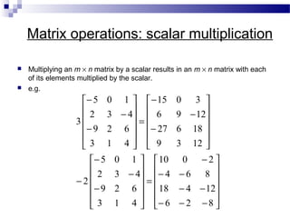
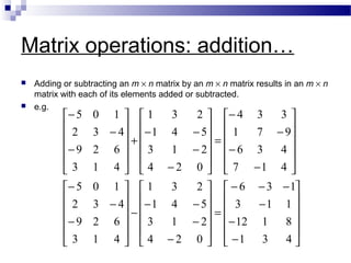
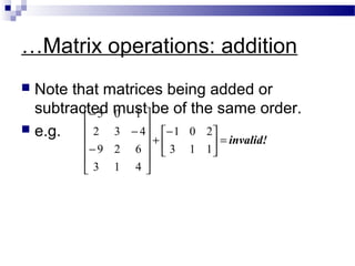
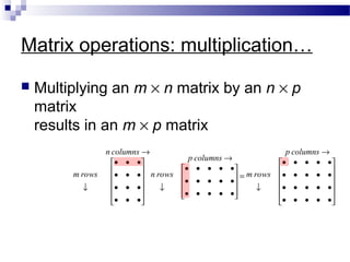
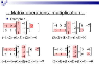
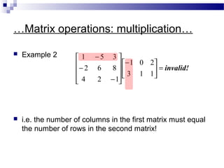
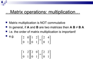
This document provides an overview of matrices and matrix operations. It defines what a matrix is and discusses matrix order and elements. It then covers basic matrix operations like scalar multiplication, addition, and multiplication. It introduces the concepts of transpose, special matrices like diagonal and triangular matrices, and the null and identity matrices. The document aims to define fundamental matrix concepts and arithmetic operations.


![43040989[1]](https://cdn.slidesharecdn.com/ss_thumbnails/430409891-100920031026-phpapp02-thumbnail.jpg?width=640&height=640&fit=bounds)


