Download as PDF, PPTX
![Images/cinvestav
A Remarkable Revenant
This algorithm has been used by many communities
Discovered and rediscovered, until 1985 it reached the AI community
[1]
Basically
The Basis of the modern neural networks
4 / 158](https://image.slidesharecdn.com/05backpropagationautomaticdifferentiation-191105020025/75/05-backpropagation-automatic_differentiation-4-2048.jpg)
![Images/cinvestav
A Remarkable Revenant
This algorithm has been used by many communities
Discovered and rediscovered, until 1985 it reached the AI community
[1]
Basically
The Basis of the modern neural networks
4 / 158](https://image.slidesharecdn.com/05backpropagationautomaticdifferentiation-191105020025/75/05-backpropagation-automatic_differentiation-5-2048.jpg)
![Images/cinvestav
Extended Network
The computation of the error by the network [2]
NETWORK
8 / 158](https://image.slidesharecdn.com/05backpropagationautomaticdifferentiation-191105020025/75/05-backpropagation-automatic_differentiation-12-2048.jpg)


![Images/cinvestav
Now a Historical Perspective
The idea of a Graph Structure was proposed by Raul Rojas
“Neural Networks - A Systematic Introduction” by Raul Rojas in
1996...
TensorFlow was initially released in November 9, 2015
Originally an inception of the project “Google Brain” (Circa 2011)
So TensorFlow started around 2012-2013 with internal development
and DNNResearch’s code (Hinton’s Company)
However, the graph idea was introduced in 2002 in torch, the basis of
Pytorch (Circa 2016)
One of the creators, Samy Bengio, is the brother of Joshua Bengio [3]
34 / 158](https://image.slidesharecdn.com/05backpropagationautomaticdifferentiation-191105020025/75/05-backpropagation-automatic_differentiation-62-2048.jpg)
![Images/cinvestav
Now a Historical Perspective
The idea of a Graph Structure was proposed by Raul Rojas
“Neural Networks - A Systematic Introduction” by Raul Rojas in
1996...
TensorFlow was initially released in November 9, 2015
Originally an inception of the project “Google Brain” (Circa 2011)
So TensorFlow started around 2012-2013 with internal development
and DNNResearch’s code (Hinton’s Company)
However, the graph idea was introduced in 2002 in torch, the basis of
Pytorch (Circa 2016)
One of the creators, Samy Bengio, is the brother of Joshua Bengio [3]
34 / 158](https://image.slidesharecdn.com/05backpropagationautomaticdifferentiation-191105020025/75/05-backpropagation-automatic_differentiation-63-2048.jpg)
![Images/cinvestav
Now a Historical Perspective
The idea of a Graph Structure was proposed by Raul Rojas
“Neural Networks - A Systematic Introduction” by Raul Rojas in
1996...
TensorFlow was initially released in November 9, 2015
Originally an inception of the project “Google Brain” (Circa 2011)
So TensorFlow started around 2012-2013 with internal development
and DNNResearch’s code (Hinton’s Company)
However, the graph idea was introduced in 2002 in torch, the basis of
Pytorch (Circa 2016)
One of the creators, Samy Bengio, is the brother of Joshua Bengio [3]
34 / 158](https://image.slidesharecdn.com/05backpropagationautomaticdifferentiation-191105020025/75/05-backpropagation-automatic_differentiation-64-2048.jpg)
![Images/cinvestav
Now a Historical Perspective
The idea of a Graph Structure was proposed by Raul Rojas
“Neural Networks - A Systematic Introduction” by Raul Rojas in
1996...
TensorFlow was initially released in November 9, 2015
Originally an inception of the project “Google Brain” (Circa 2011)
So TensorFlow started around 2012-2013 with internal development
and DNNResearch’s code (Hinton’s Company)
However, the graph idea was introduced in 2002 in torch, the basis of
Pytorch (Circa 2016)
One of the creators, Samy Bengio, is the brother of Joshua Bengio [3]
34 / 158](https://image.slidesharecdn.com/05backpropagationautomaticdifferentiation-191105020025/75/05-backpropagation-automatic_differentiation-65-2048.jpg)
![Images/cinvestav
Backpropagation a little brother of Automatic
Differentiation (AD)
We have a crude way to obtain derivatives [4, 5, 6][7]
D+hf (x) ≈
f (x + h) − f (x)
2h
or D hf (x) ≈
f (x + h) − f (x − h)
2h
Huge Problems
If h is small, then cancellation error reduces the number of significant
figures in D+hf (x).
if h is not small, then truncation errors (terms such as h2f (x))
become significant.
Even if h is optimally chosen, the values of D+hf (x) and D hf (x)
will be accurate to only about 1
2 or 2
3 of the significant digits of f.
36 / 158](https://image.slidesharecdn.com/05backpropagationautomaticdifferentiation-191105020025/75/05-backpropagation-automatic_differentiation-67-2048.jpg)
![Images/cinvestav
Backpropagation a little brother of Automatic
Differentiation (AD)
We have a crude way to obtain derivatives [4, 5, 6][7]
D+hf (x) ≈
f (x + h) − f (x)
2h
or D hf (x) ≈
f (x + h) − f (x − h)
2h
Huge Problems
If h is small, then cancellation error reduces the number of significant
figures in D+hf (x).
if h is not small, then truncation errors (terms such as h2f (x))
become significant.
Even if h is optimally chosen, the values of D+hf (x) and D hf (x)
will be accurate to only about 1
2 or 2
3 of the significant digits of f.
36 / 158](https://image.slidesharecdn.com/05backpropagationautomaticdifferentiation-191105020025/75/05-backpropagation-automatic_differentiation-68-2048.jpg)
![Images/cinvestav
Backpropagation a little brother of Automatic
Differentiation (AD)
We have a crude way to obtain derivatives [4, 5, 6][7]
D+hf (x) ≈
f (x + h) − f (x)
2h
or D hf (x) ≈
f (x + h) − f (x − h)
2h
Huge Problems
If h is small, then cancellation error reduces the number of significant
figures in D+hf (x).
if h is not small, then truncation errors (terms such as h2f (x))
become significant.
Even if h is optimally chosen, the values of D+hf (x) and D hf (x)
will be accurate to only about 1
2 or 2
3 of the significant digits of f.
36 / 158](https://image.slidesharecdn.com/05backpropagationautomaticdifferentiation-191105020025/75/05-backpropagation-automatic_differentiation-69-2048.jpg)
![Images/cinvestav
Backpropagation a little brother of Automatic
Differentiation (AD)
We have a crude way to obtain derivatives [4, 5, 6][7]
D+hf (x) ≈
f (x + h) − f (x)
2h
or D hf (x) ≈
f (x + h) − f (x − h)
2h
Huge Problems
If h is small, then cancellation error reduces the number of significant
figures in D+hf (x).
if h is not small, then truncation errors (terms such as h2f (x))
become significant.
Even if h is optimally chosen, the values of D+hf (x) and D hf (x)
will be accurate to only about 1
2 or 2
3 of the significant digits of f.
36 / 158](https://image.slidesharecdn.com/05backpropagationautomaticdifferentiation-191105020025/75/05-backpropagation-automatic_differentiation-70-2048.jpg)


![Images/cinvestav
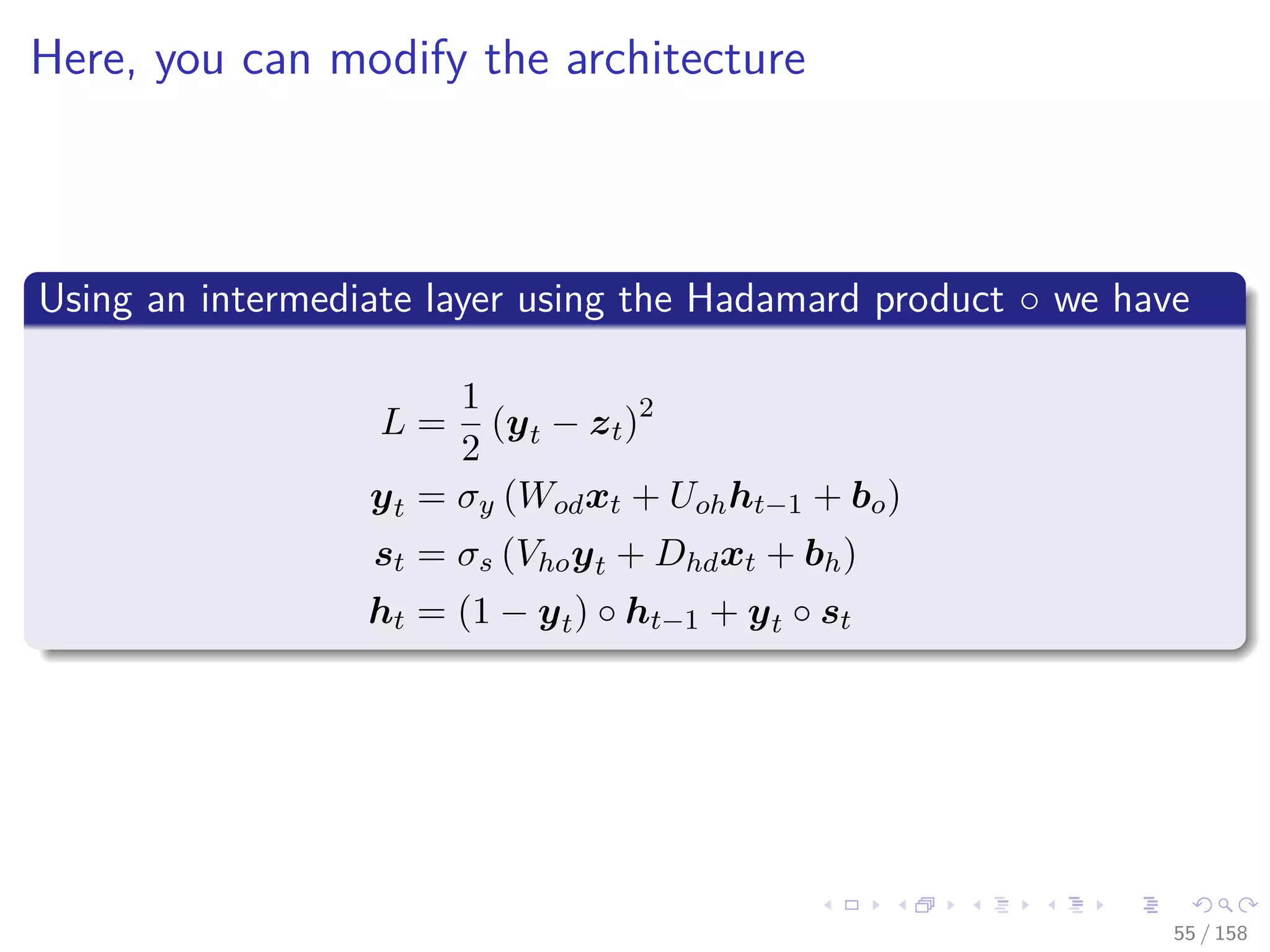
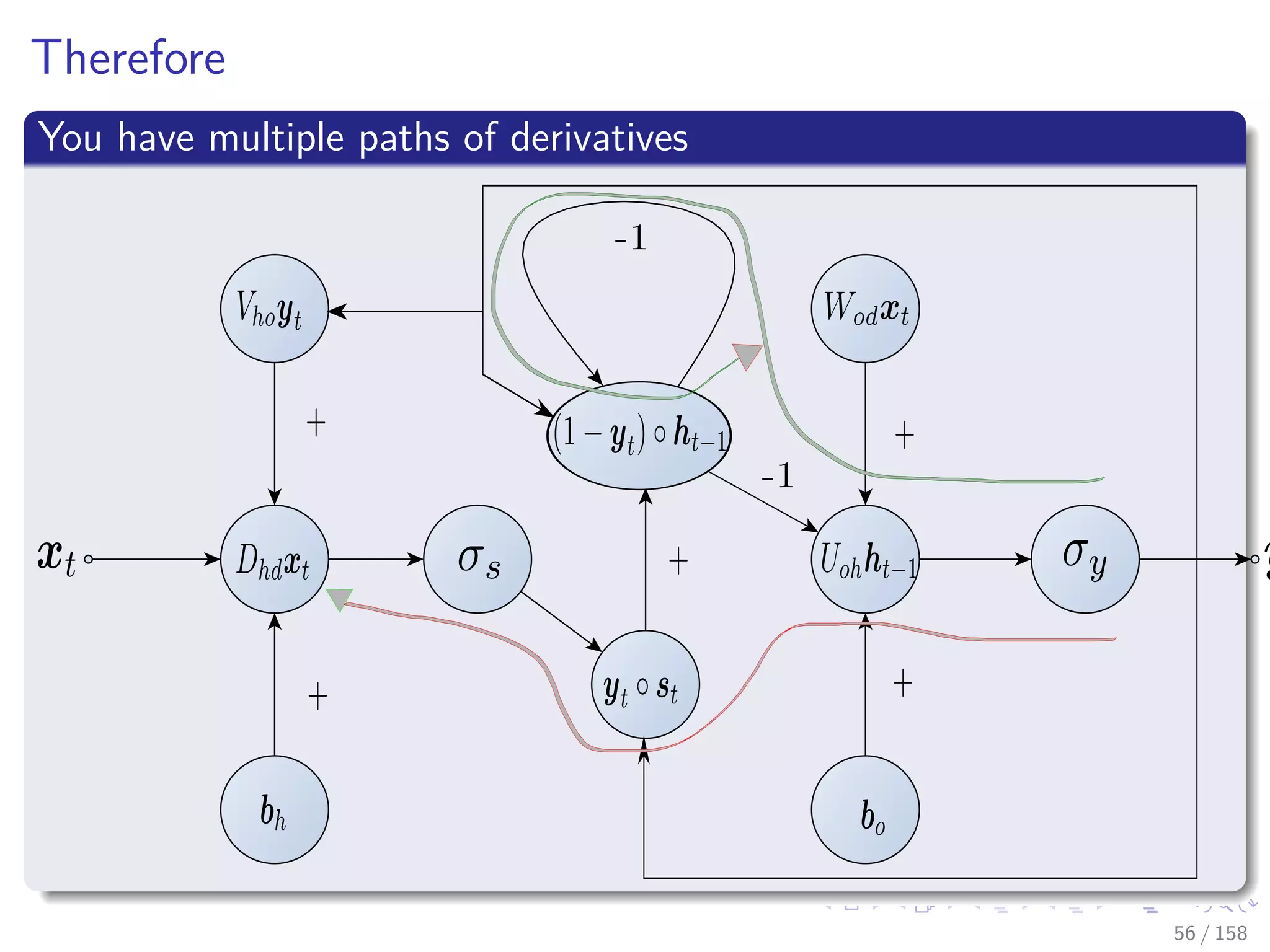
RNN Example
When you look at the recurrent neural network Elman [8]
ht = σh (Wsdxt + Ushht−1 + bh)
yt = σy (Vosht)
L =
1
2
(yt − zt)2
Here if you do blind AD sooner or later you have
∂ht
∂ht−1
×
∂ht−1
∂ht−2
×
∂ht−2
∂ht−3
× ... ×
∂hk+1
∂hk
This is known as Back Propagation Through Time (BPTT)
This is a problem given
The Vanishing Gradient or Exploding Gradient
54 / 158](https://image.slidesharecdn.com/05backpropagationautomaticdifferentiation-191105020025/75/05-backpropagation-automatic_differentiation-104-2048.jpg)
![Images/cinvestav
RNN Example
When you look at the recurrent neural network Elman [8]
ht = σh (Wsdxt + Ushht−1 + bh)
yt = σy (Vosht)
L =
1
2
(yt − zt)2
Here if you do blind AD sooner or later you have
∂ht
∂ht−1
×
∂ht−1
∂ht−2
×
∂ht−2
∂ht−3
× ... ×
∂hk+1
∂hk
This is known as Back Propagation Through Time (BPTT)
This is a problem given
The Vanishing Gradient or Exploding Gradient
54 / 158](https://image.slidesharecdn.com/05backpropagationautomaticdifferentiation-191105020025/75/05-backpropagation-automatic_differentiation-105-2048.jpg)
![Images/cinvestav
RNN Example
When you look at the recurrent neural network Elman [8]
ht = σh (Wsdxt + Ushht−1 + bh)
yt = σy (Vosht)
L =
1
2
(yt − zt)2
Here if you do blind AD sooner or later you have
∂ht
∂ht−1
×
∂ht−1
∂ht−2
×
∂ht−2
∂ht−3
× ... ×
∂hk+1
∂hk
This is known as Back Propagation Through Time (BPTT)
This is a problem given
The Vanishing Gradient or Exploding Gradient
54 / 158](https://image.slidesharecdn.com/05backpropagationautomaticdifferentiation-191105020025/75/05-backpropagation-automatic_differentiation-106-2048.jpg)


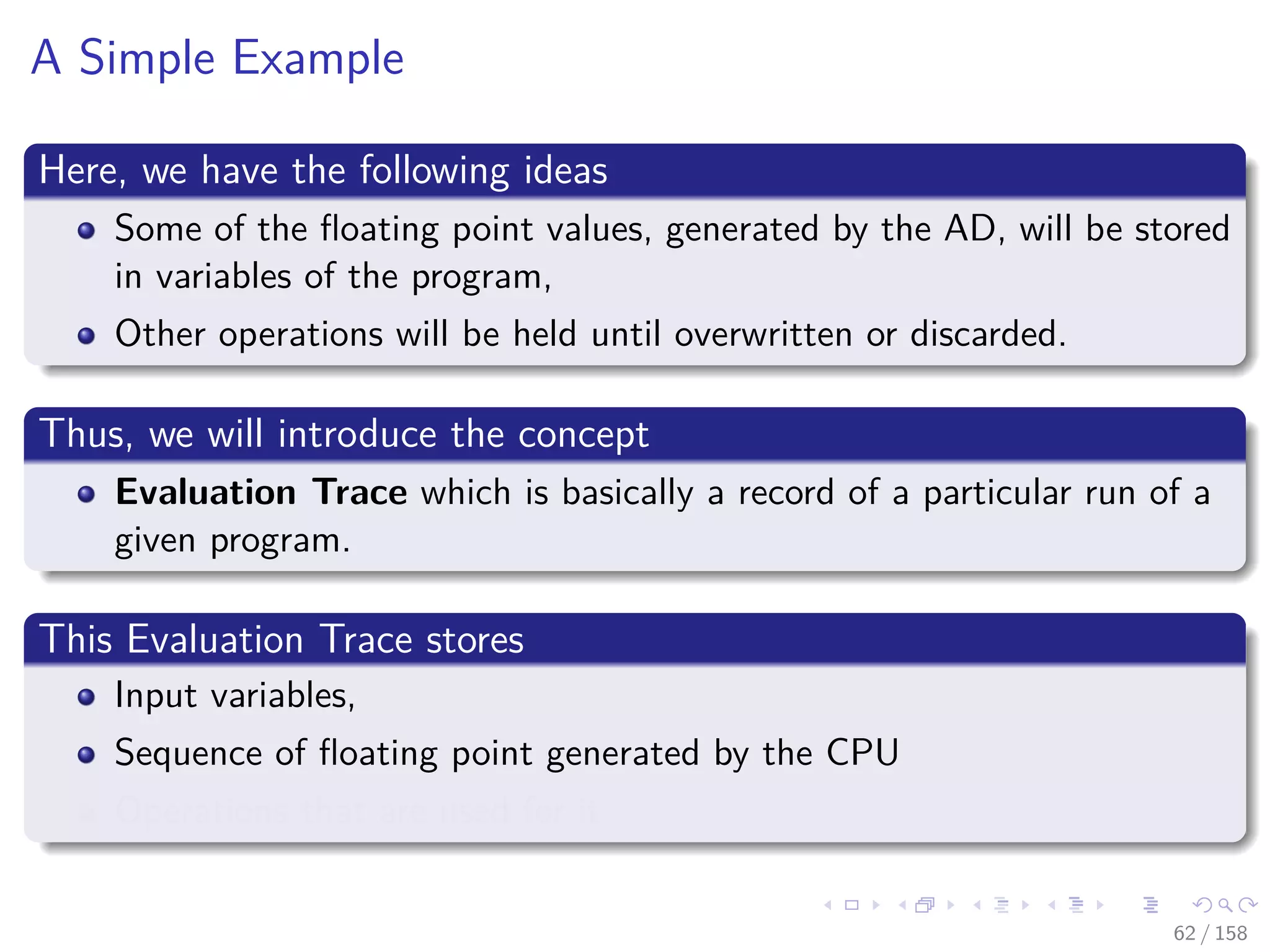
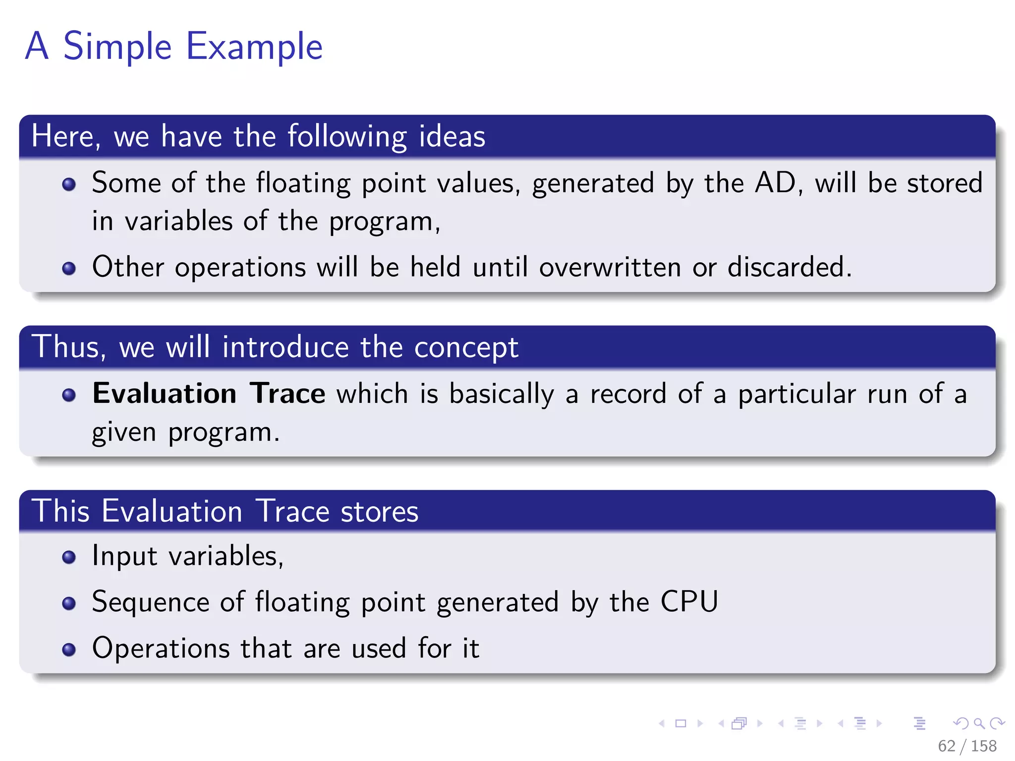
![Images/cinvestav
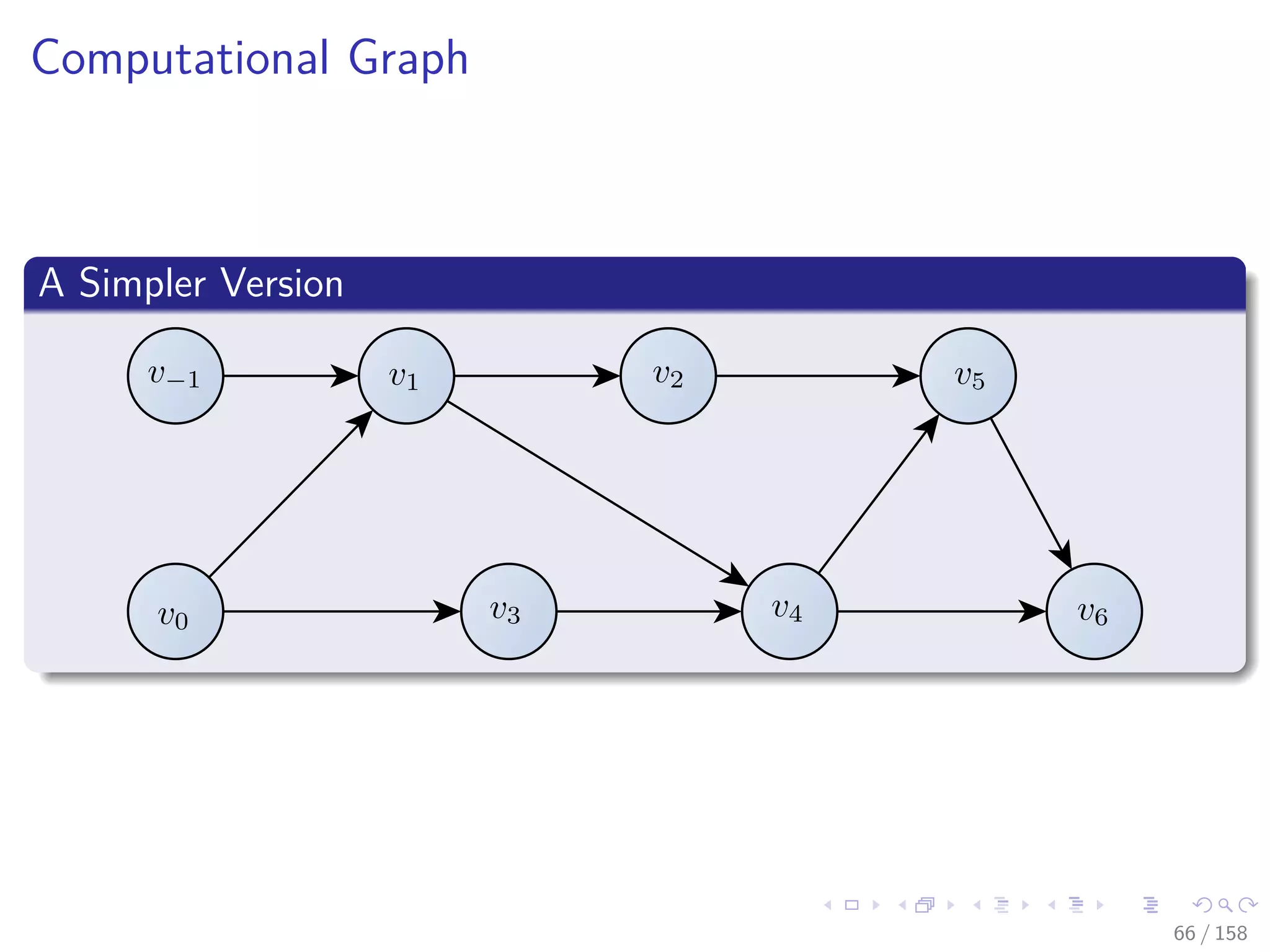
Please take a look at section in Chapter 2 A Framework for
Evaluating Functions
At the book [7]
Andreas Griewank and Andrea Walther, Evaluating derivatives:
principles and techniques of algorithmic differentiation vol. 105,
(Siam, 2008).
67 / 158](https://image.slidesharecdn.com/05backpropagationautomaticdifferentiation-191105020025/75/05-backpropagation-automatic_differentiation-130-2048.jpg)

![Images/cinvestav
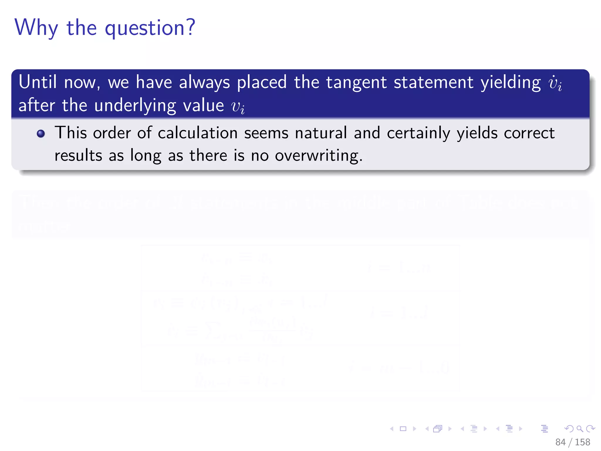
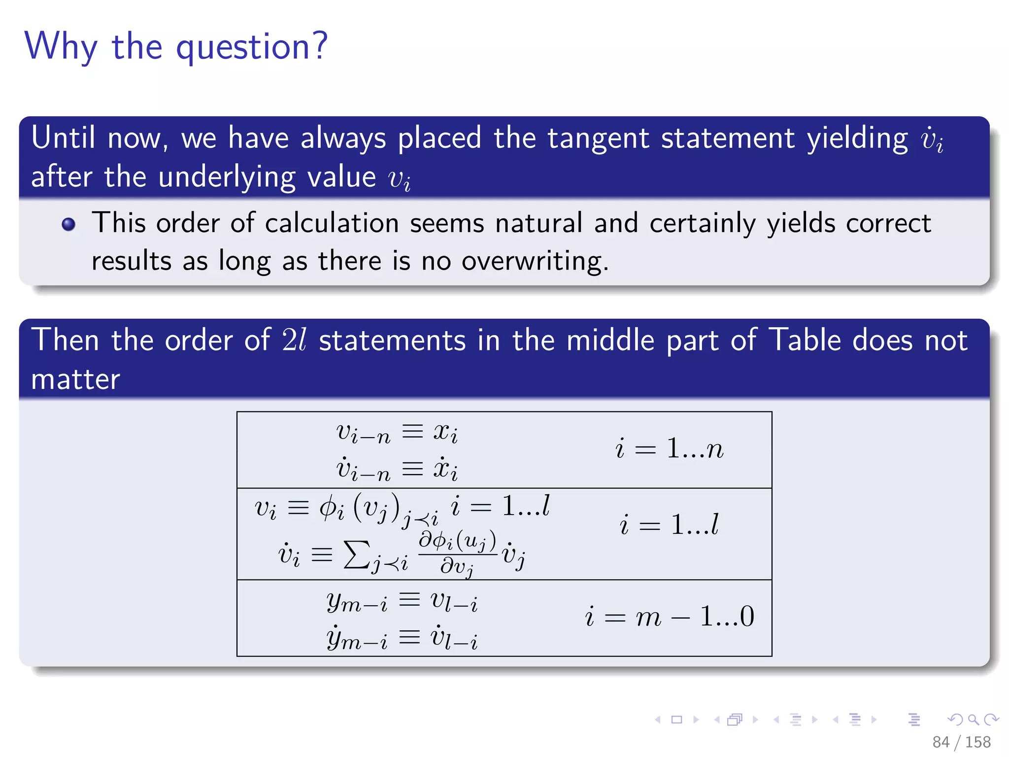
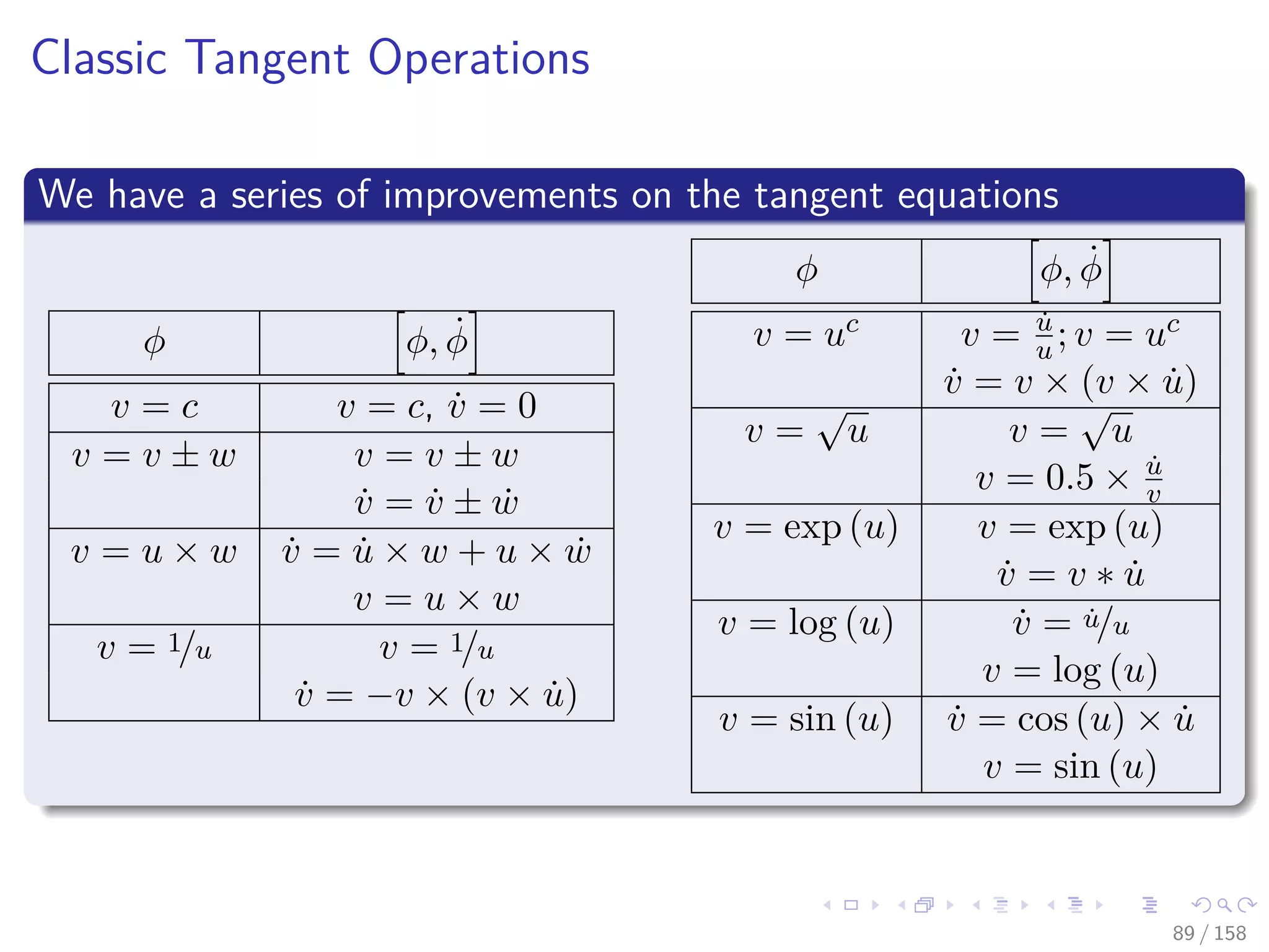
Then
The value of ˙vi = ˙φi (ui, ˙ui) it will incorrect
Once we update vi = φi (ui)
ADIFOR and Tapenade [9, 5]
They put the derivative statement ahead of the original assignment
and update before the erasing the original statement.
On the other hand
For most univariate functions v = φ (u) is better to obtain the
undifferentiated value first
Then to use it into the tangent function ˙φ
87 / 158](https://image.slidesharecdn.com/05backpropagationautomaticdifferentiation-191105020025/75/05-backpropagation-automatic_differentiation-165-2048.jpg)
![Images/cinvestav
Then
The value of ˙vi = ˙φi (ui, ˙ui) it will incorrect
Once we update vi = φi (ui)
ADIFOR and Tapenade [9, 5]
They put the derivative statement ahead of the original assignment
and update before the erasing the original statement.
On the other hand
For most univariate functions v = φ (u) is better to obtain the
undifferentiated value first
Then to use it into the tangent function ˙φ
87 / 158](https://image.slidesharecdn.com/05backpropagationautomaticdifferentiation-191105020025/75/05-backpropagation-automatic_differentiation-166-2048.jpg)
![Images/cinvestav
Then
The value of ˙vi = ˙φi (ui, ˙ui) it will incorrect
Once we update vi = φi (ui)
ADIFOR and Tapenade [9, 5]
They put the derivative statement ahead of the original assignment
and update before the erasing the original statement.
On the other hand
For most univariate functions v = φ (u) is better to obtain the
undifferentiated value first
Then to use it into the tangent function ˙φ
87 / 158](https://image.slidesharecdn.com/05backpropagationautomaticdifferentiation-191105020025/75/05-backpropagation-automatic_differentiation-167-2048.jpg)
![Images/cinvestav
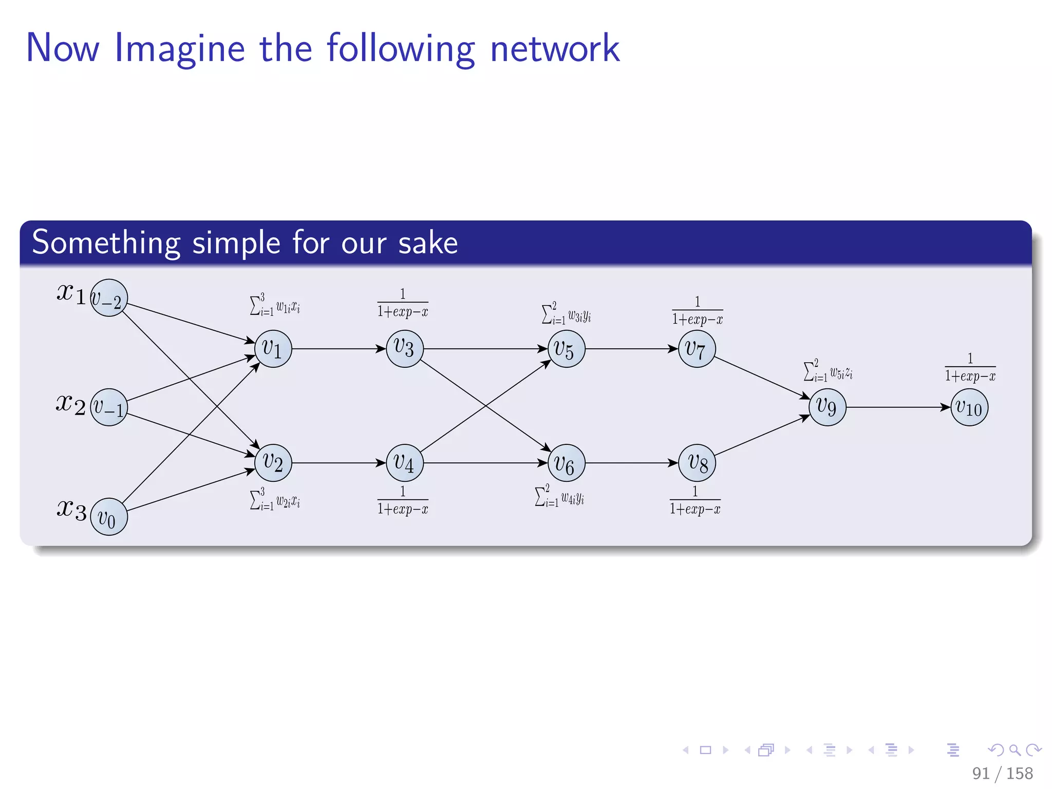
Forward mode to get gradient of x1
v−11 = w11, ..., v−6 = w16, v−5 = w21, ..., v−2 = w24, v−1 = v31, v−1 = w41
˙v−11 = 1, ˙v−10 = 0, ..., ˙v0 = 0
v1 =
3
i=1
w1ixi , ˙v1 = x1
v2 =
3
i=1
w2ixi , ˙v2 = 0
v3 = 1
1+exp(−v1)
, ˙v3 = v3 [1 − v3] x11
v4 = 1
1+exp(−v2)
, ˙v4 = 0
v5 =
3
i=1
w3ivi, ˙v5 = w31 × ˙v3
v6 =
3
i=1
w4ivi, ˙v6 = w41 × ˙v3
v7 = 1
1+exp(−v5)
, ˙v7 = v7 [1 − v7] × ˙v5
v8 = 1
1+exp(−v6)
, ˙v8 = v8 [1 − v8] × ˙v6
v9 =
2
i=1
w5ivi, ˙v9 = w51 × ˙v7 + w32 × ˙v8
v10 = 1
1+exp(−v9)
, ˙v10 = v10 [1 − v10] × ˙v9
92 / 158](https://image.slidesharecdn.com/05backpropagationautomaticdifferentiation-191105020025/75/05-backpropagation-automatic_differentiation-173-2048.jpg)
![Images/cinvestav
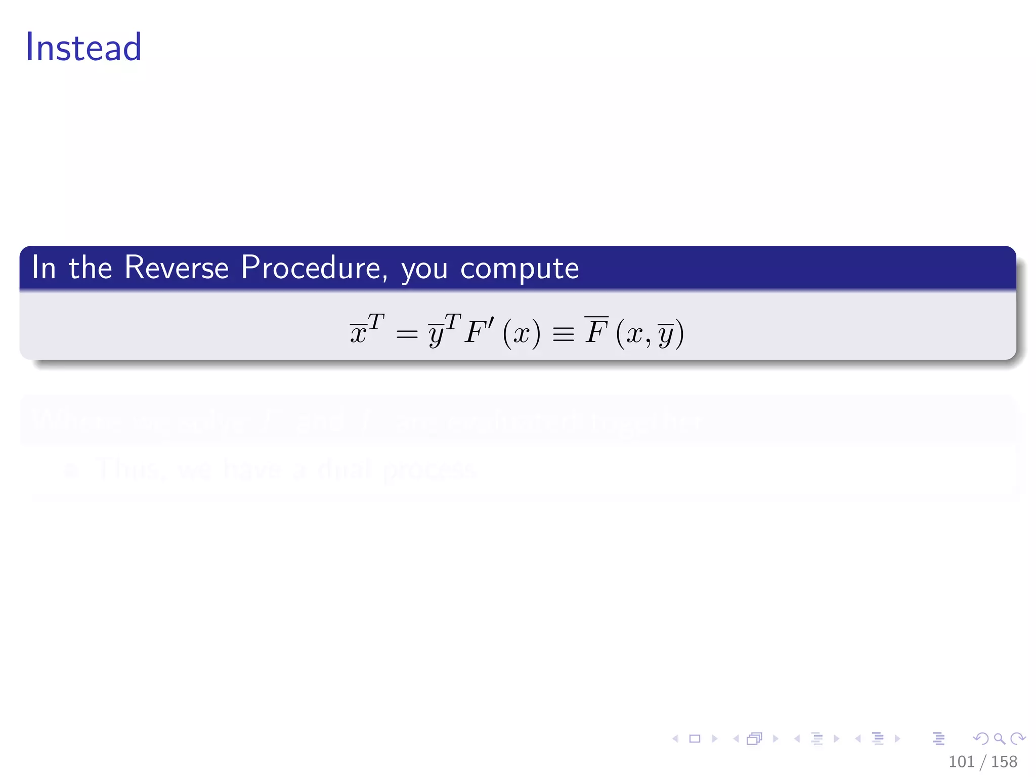
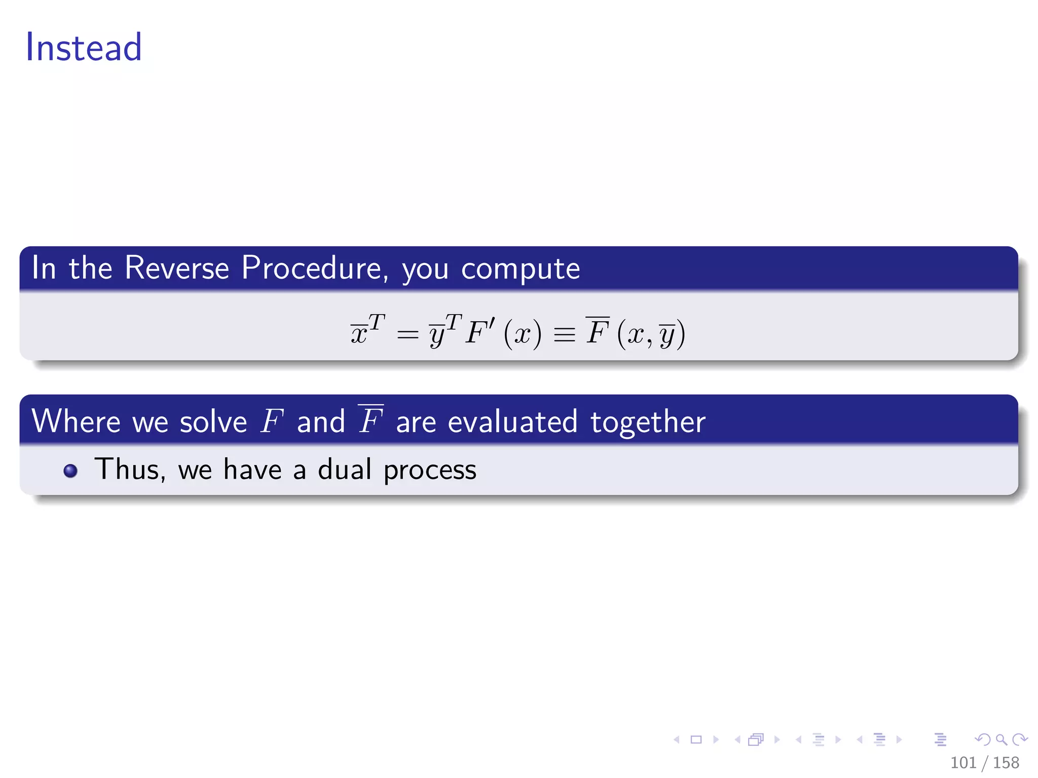
We choose instead an output variable
We use the term “reverse mode” for this technique
Because the label “backward differentiation” is well established
[10, 11].
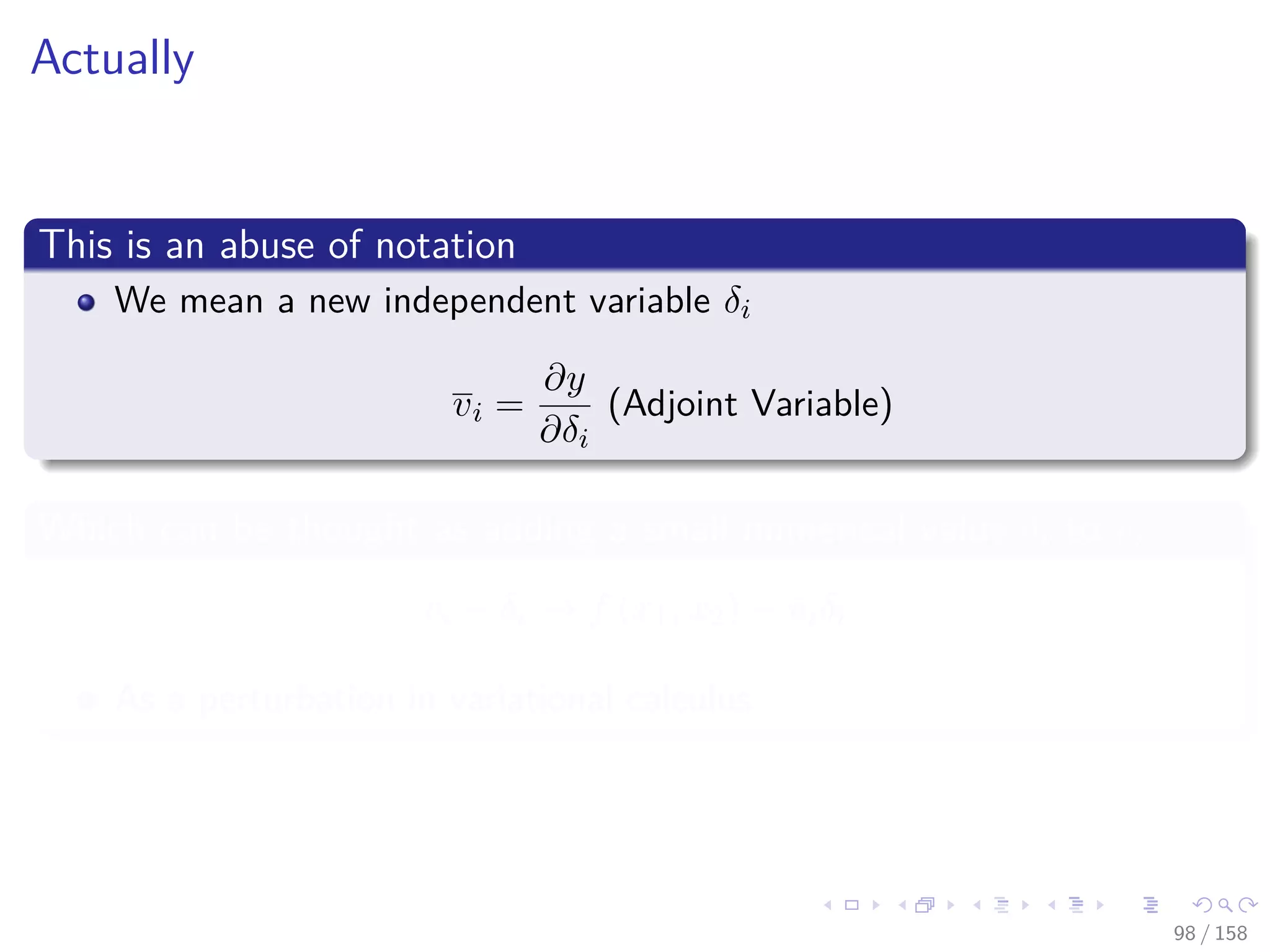
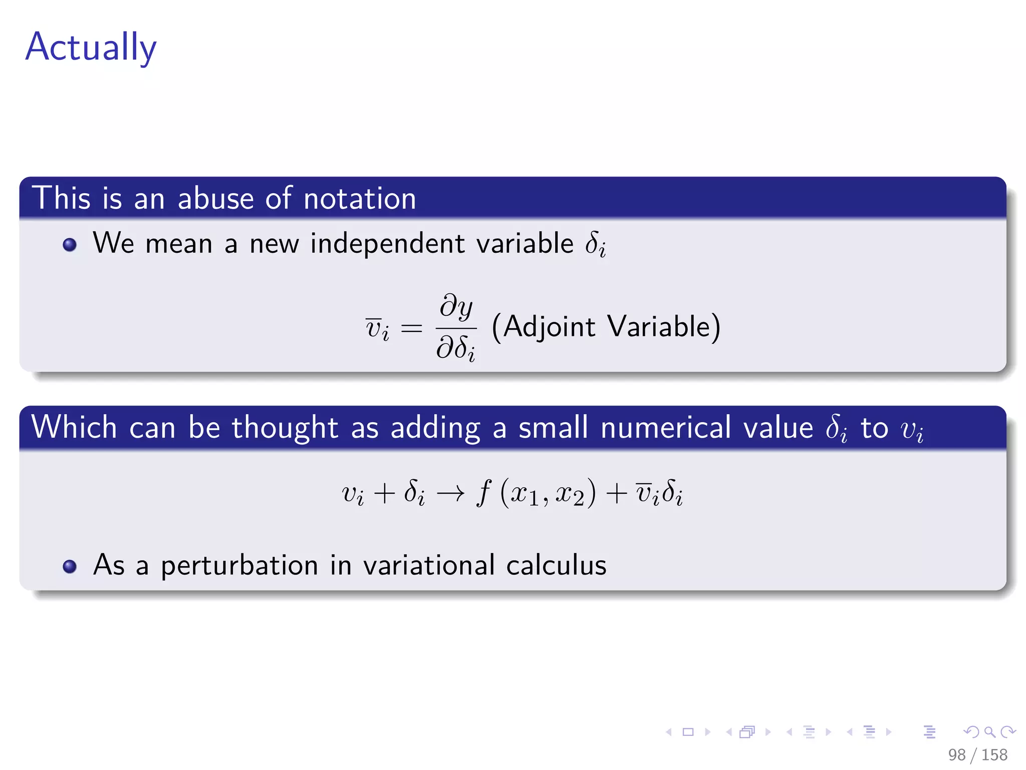
Therefore, for an output f (x1, x2)
We have for each variable v1
vi =
∂y
∂vi
(Adjoint Variable)
97 / 158](https://image.slidesharecdn.com/05backpropagationautomaticdifferentiation-191105020025/75/05-backpropagation-automatic_differentiation-180-2048.jpg)
![Images/cinvestav
We choose instead an output variable
We use the term “reverse mode” for this technique
Because the label “backward differentiation” is well established
[10, 11].
Therefore, for an output f (x1, x2)
We have for each variable v1
vi =
∂y
∂vi
(Adjoint Variable)
97 / 158](https://image.slidesharecdn.com/05backpropagationautomaticdifferentiation-191105020025/75/05-backpropagation-automatic_differentiation-181-2048.jpg)
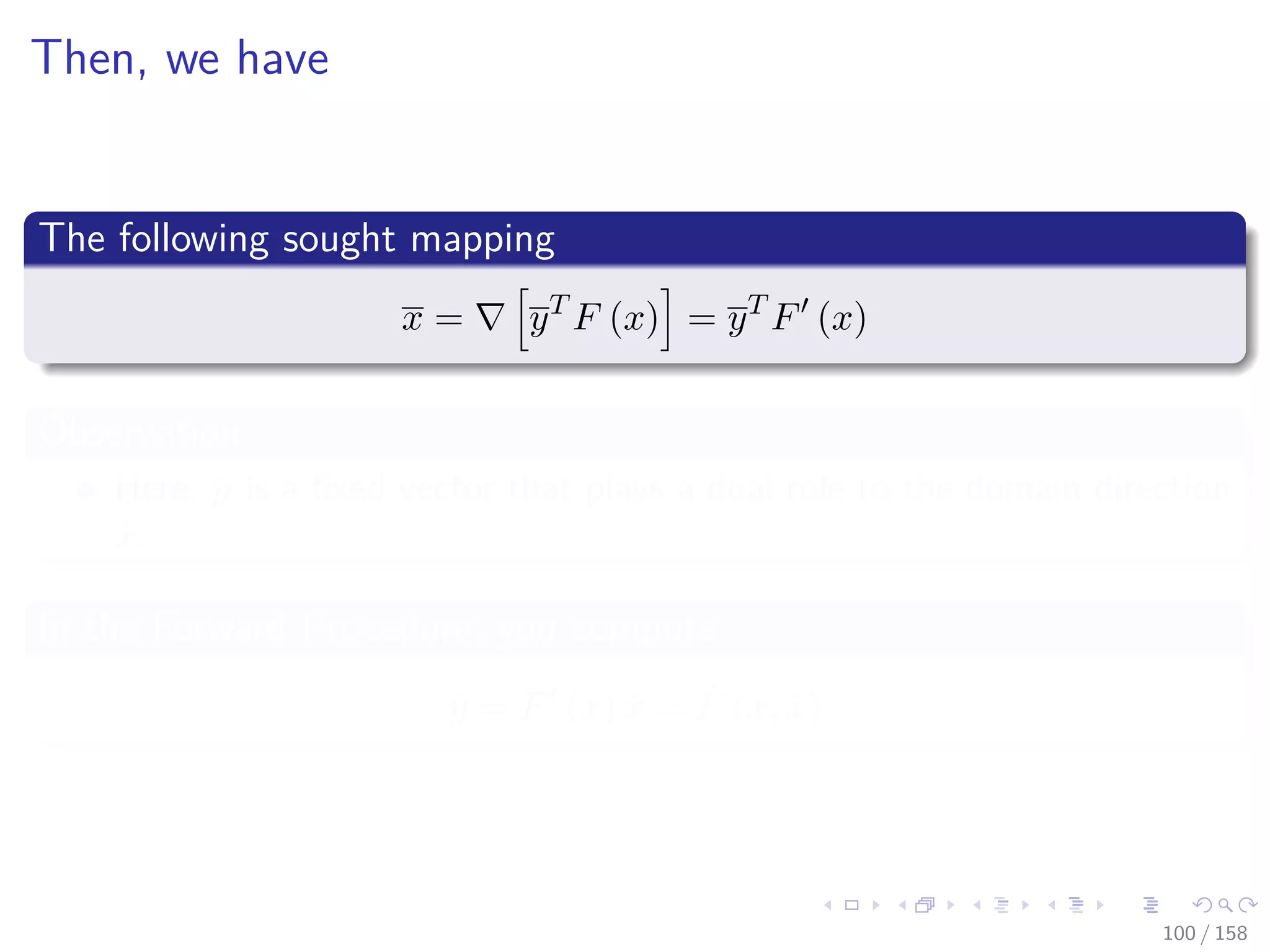
![Images/cinvestav
Therefore
When m = 1, then F = f is scaler-valued
We obtain y = 1 ∈ R the familiar gradient f (x) = yT F (x).
Something Notable
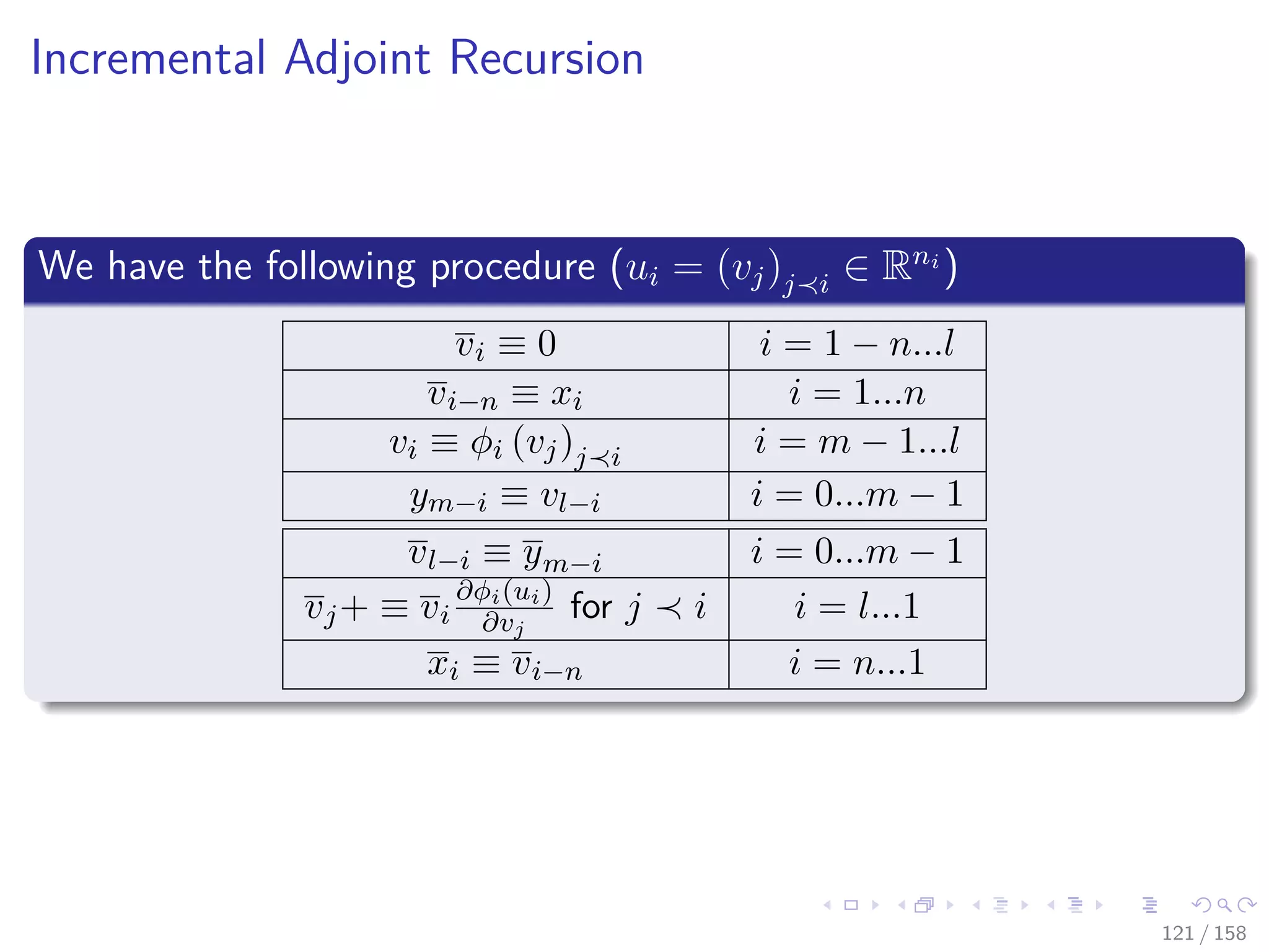
We will look only at the main procedure of Incremental Adjoint
Recursion
Please take a look at section in Derivation by Matrix-Product
Reversal
At the book [7]
Andreas Griewank and Andrea Walther, Evaluating derivatives:
principles and techniques of algorithmic differentiation vol. 105,
(Siam, 2008).
107 / 158](https://image.slidesharecdn.com/05backpropagationautomaticdifferentiation-191105020025/75/05-backpropagation-automatic_differentiation-195-2048.jpg)
![Images/cinvestav
Therefore
When m = 1, then F = f is scaler-valued
We obtain y = 1 ∈ R the familiar gradient f (x) = yT F (x).
Something Notable
We will look only at the main procedure of Incremental Adjoint
Recursion
Please take a look at section in Derivation by Matrix-Product
Reversal
At the book [7]
Andreas Griewank and Andrea Walther, Evaluating derivatives:
principles and techniques of algorithmic differentiation vol. 105,
(Siam, 2008).
107 / 158](https://image.slidesharecdn.com/05backpropagationautomaticdifferentiation-191105020025/75/05-backpropagation-automatic_differentiation-196-2048.jpg)
![Images/cinvestav
Therefore
When m = 1, then F = f is scaler-valued
We obtain y = 1 ∈ R the familiar gradient f (x) = yT F (x).
Something Notable
We will look only at the main procedure of Incremental Adjoint
Recursion
Please take a look at section in Derivation by Matrix-Product
Reversal
At the book [7]
Andreas Griewank and Andrea Walther, Evaluating derivatives:
principles and techniques of algorithmic differentiation vol. 105,
(Siam, 2008).
107 / 158](https://image.slidesharecdn.com/05backpropagationautomaticdifferentiation-191105020025/75/05-backpropagation-automatic_differentiation-197-2048.jpg)
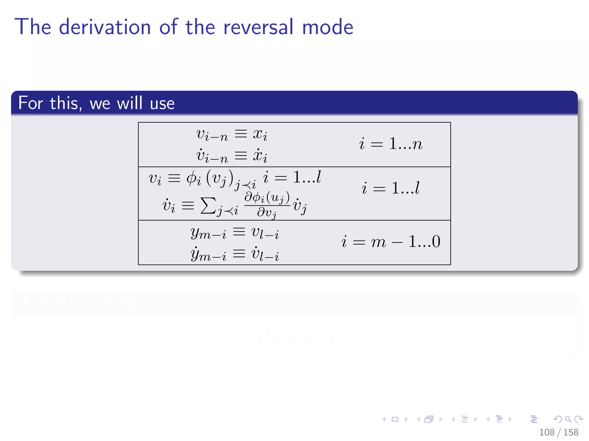
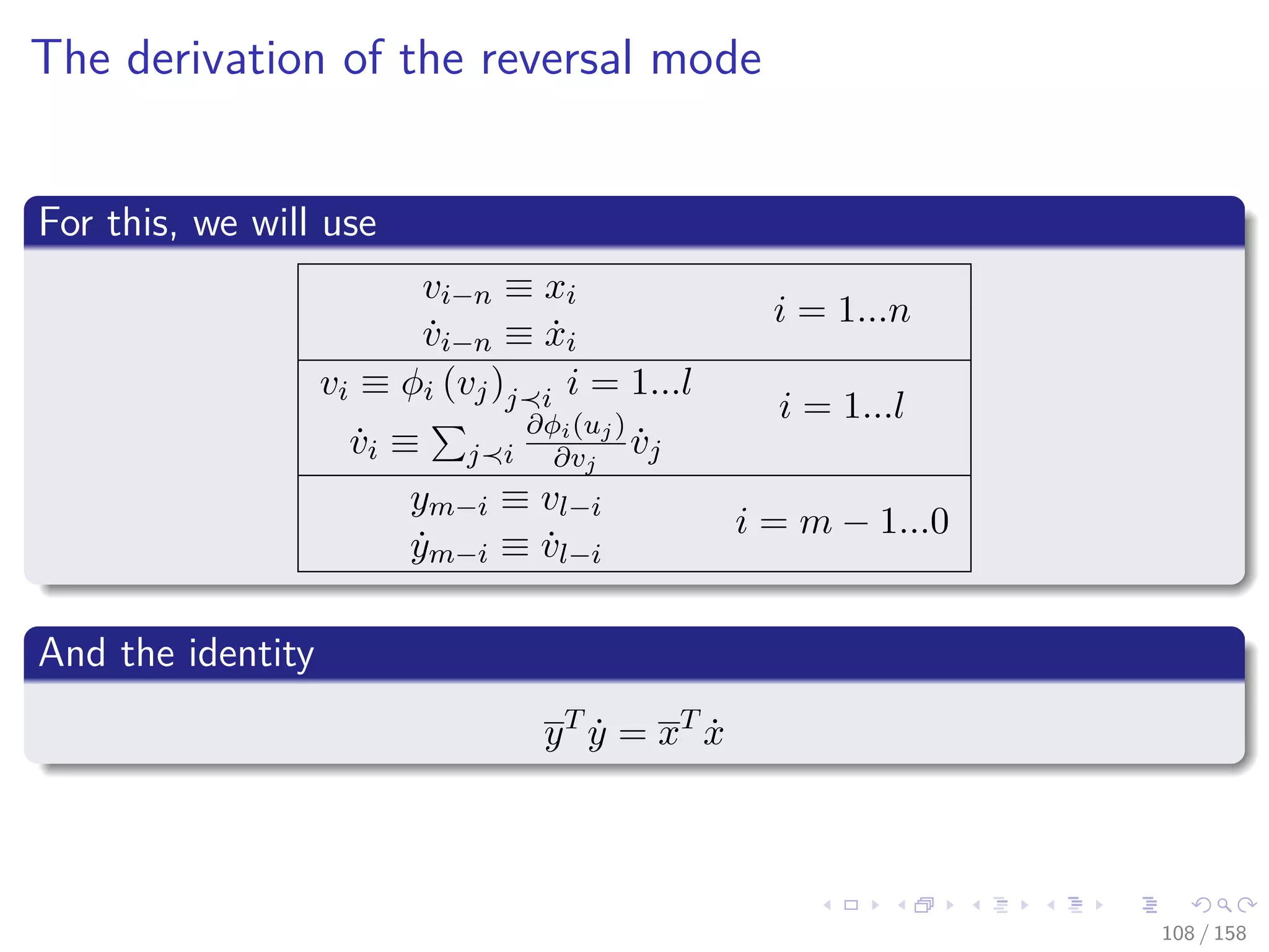
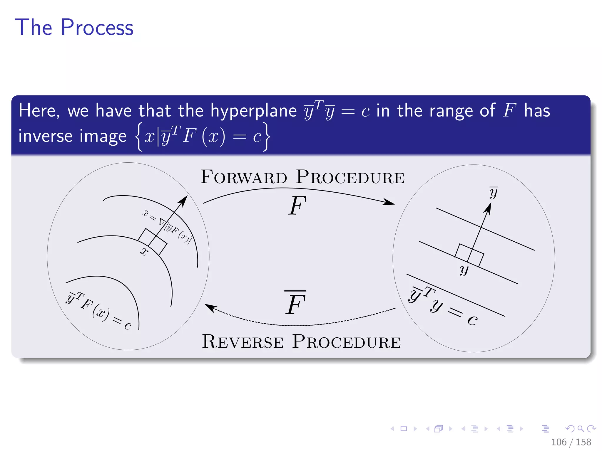
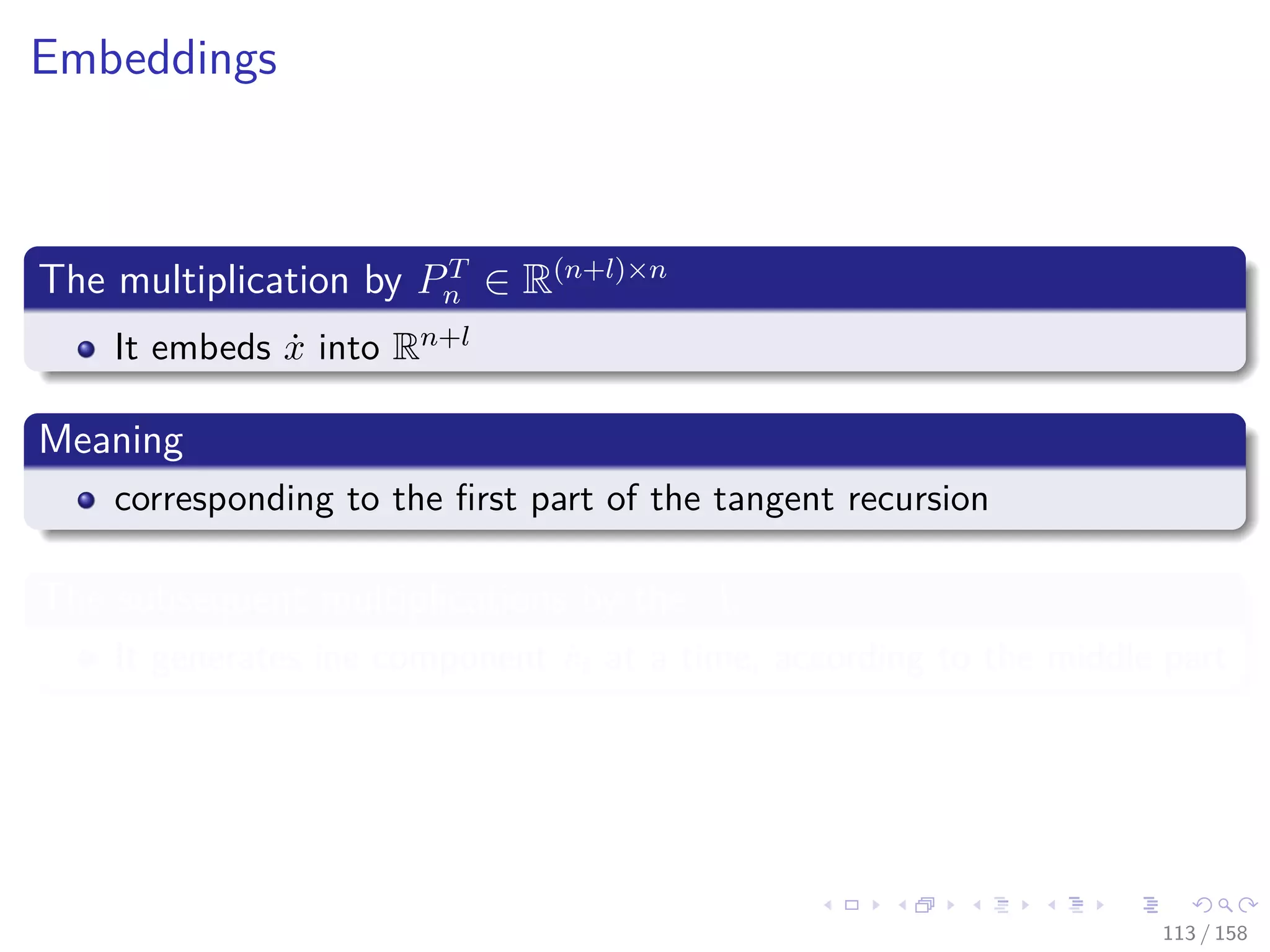
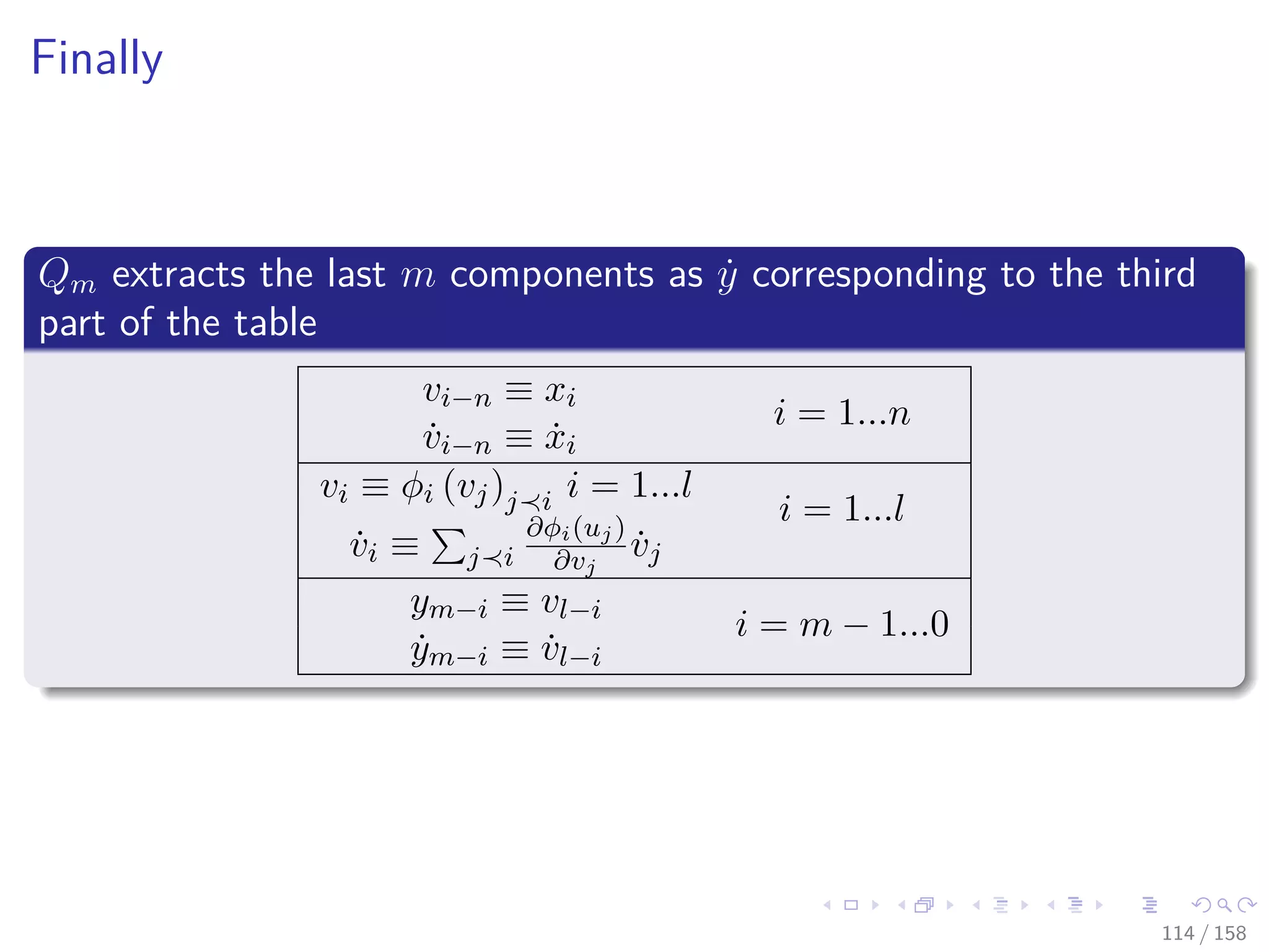
![Images/cinvestav
Now, using the state transformation Φ
We map from x to y = F (x) as the composition
y = QmΦl ◦ Φl−1 ◦ · · · ◦ Φ2 ◦ Φ1 PT
n x
Where Pn ≡ [I, 0, ..., 0] ∈ Rn×(n+l) and Qm ≡ [0, 0, ..., I] ∈ Rm×(n+l)
They are matrices that project an arbitrary (n + l)-vector
Onto its first n and last m components.
109 / 158](https://image.slidesharecdn.com/05backpropagationautomaticdifferentiation-191105020025/75/05-backpropagation-automatic_differentiation-200-2048.jpg)
![Images/cinvestav
Now, using the state transformation Φ
We map from x to y = F (x) as the composition
y = QmΦl ◦ Φl−1 ◦ · · · ◦ Φ2 ◦ Φ1 PT
n x
Where Pn ≡ [I, 0, ..., 0] ∈ Rn×(n+l) and Qm ≡ [0, 0, ..., I] ∈ Rm×(n+l)
They are matrices that project an arbitrary (n + l)-vector
Onto its first n and last m components.
109 / 158](https://image.slidesharecdn.com/05backpropagationautomaticdifferentiation-191105020025/75/05-backpropagation-automatic_differentiation-201-2048.jpg)
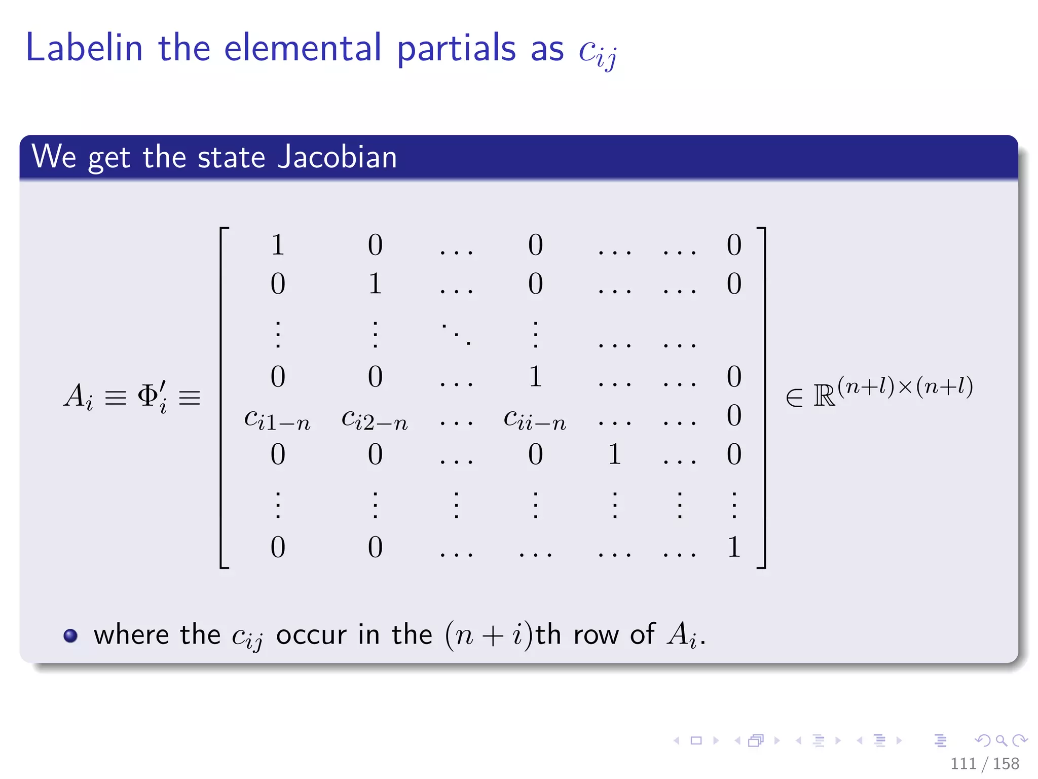
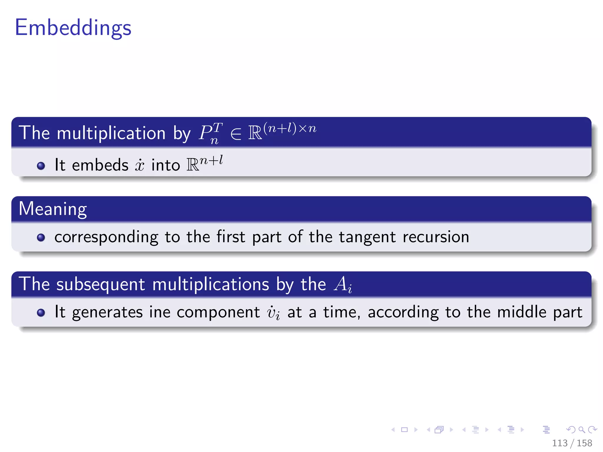
![Images/cinvestav
Remarks
The square matrices Ai are lower triangular
It may also be written as rank-one perturbations of the identity,
Ai = I + en+i [ φi (ui) − en+i]T
Where ej denotes the jth Cartesian basis vector in Rn+l
The differentiating the composition of functions
˙y = QmAlAl−1 · · · A2A1PT
n ˙x
112 / 158](https://image.slidesharecdn.com/05backpropagationautomaticdifferentiation-191105020025/75/05-backpropagation-automatic_differentiation-204-2048.jpg)
![Images/cinvestav
Remarks
The square matrices Ai are lower triangular
It may also be written as rank-one perturbations of the identity,
Ai = I + en+i [ φi (ui) − en+i]T
Where ej denotes the jth Cartesian basis vector in Rn+l
The differentiating the composition of functions
˙y = QmAlAl−1 · · · A2A1PT
n ˙x
112 / 158](https://image.slidesharecdn.com/05backpropagationautomaticdifferentiation-191105020025/75/05-backpropagation-automatic_differentiation-205-2048.jpg)
![Images/cinvestav
Then
By transposing the product we obtain the adjoint relation
x = PnAT
1 AT
2 · · · AT
l−1AT
l y
Given that
AT
i = I + [ φi (ui) − en+i] eT
n+i
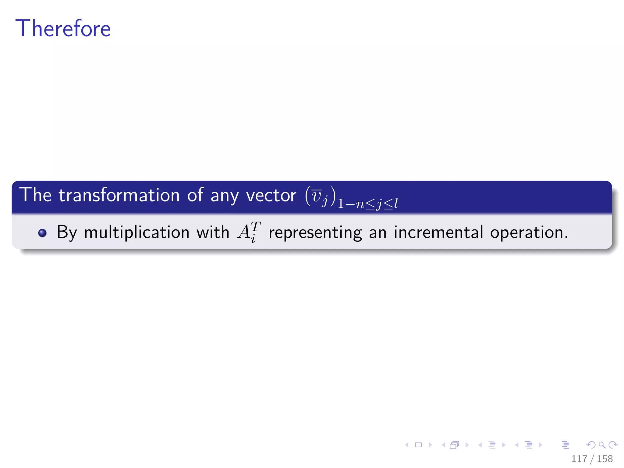
116 / 158](https://image.slidesharecdn.com/05backpropagationautomaticdifferentiation-191105020025/75/05-backpropagation-automatic_differentiation-212-2048.jpg)
![Images/cinvestav
Then
By transposing the product we obtain the adjoint relation
x = PnAT
1 AT
2 · · · AT
l−1AT
l y
Given that
AT
i = I + [ φi (ui) − en+i] eT
n+i
116 / 158](https://image.slidesharecdn.com/05backpropagationautomaticdifferentiation-191105020025/75/05-backpropagation-automatic_differentiation-213-2048.jpg)
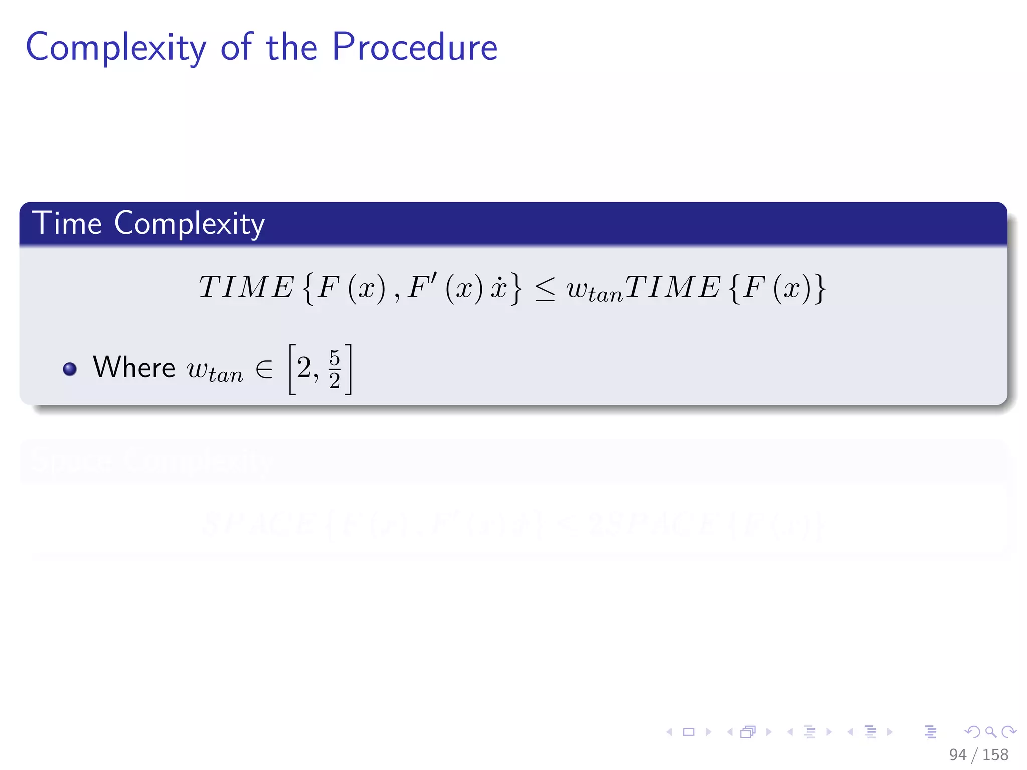
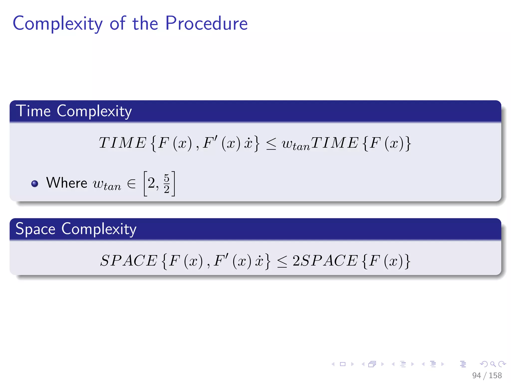
![Images/cinvestav
Complexity
Something Notable
TIME F (x) , yT
F (x) ≤ wgradTIME {F (x)}
Where wgrad ∈ [3, 4] (The cheap gradient principle)
124 / 158](https://image.slidesharecdn.com/05backpropagationautomaticdifferentiation-191105020025/75/05-backpropagation-automatic_differentiation-227-2048.jpg)

![Images/cinvestav
Nevertheless
There are many techniques to improve the efficiency and avoid
aliasing problems of these modes [12]
1 Taping for adjoint recursion
2 Caching
3 Checkpoints
4 Expression Templates
5 etc
You are invited to read more about them
Given that these techniques are already being implemented in
languages as swift...
“First-Class Automatic Differentiation in Swift: A Manifesto”
https://gist.github.com/rxwei/30ba75ce092ab3b0dce4bde1fc2c9f1d
152 / 158](https://image.slidesharecdn.com/05backpropagationautomaticdifferentiation-191105020025/75/05-backpropagation-automatic_differentiation-268-2048.jpg)
![Images/cinvestav
Nevertheless
There are many techniques to improve the efficiency and avoid
aliasing problems of these modes [12]
1 Taping for adjoint recursion
2 Caching
3 Checkpoints
4 Expression Templates
5 etc
You are invited to read more about them
Given that these techniques are already being implemented in
languages as swift...
“First-Class Automatic Differentiation in Swift: A Manifesto”
https://gist.github.com/rxwei/30ba75ce092ab3b0dce4bde1fc2c9f1d
152 / 158](https://image.slidesharecdn.com/05backpropagationautomaticdifferentiation-191105020025/75/05-backpropagation-automatic_differentiation-269-2048.jpg)
![Images/cinvestav
Between Two Extremes
Something Notable
Forward and reverse accumulation are just two (extreme) ways of
traversing the chain rule.
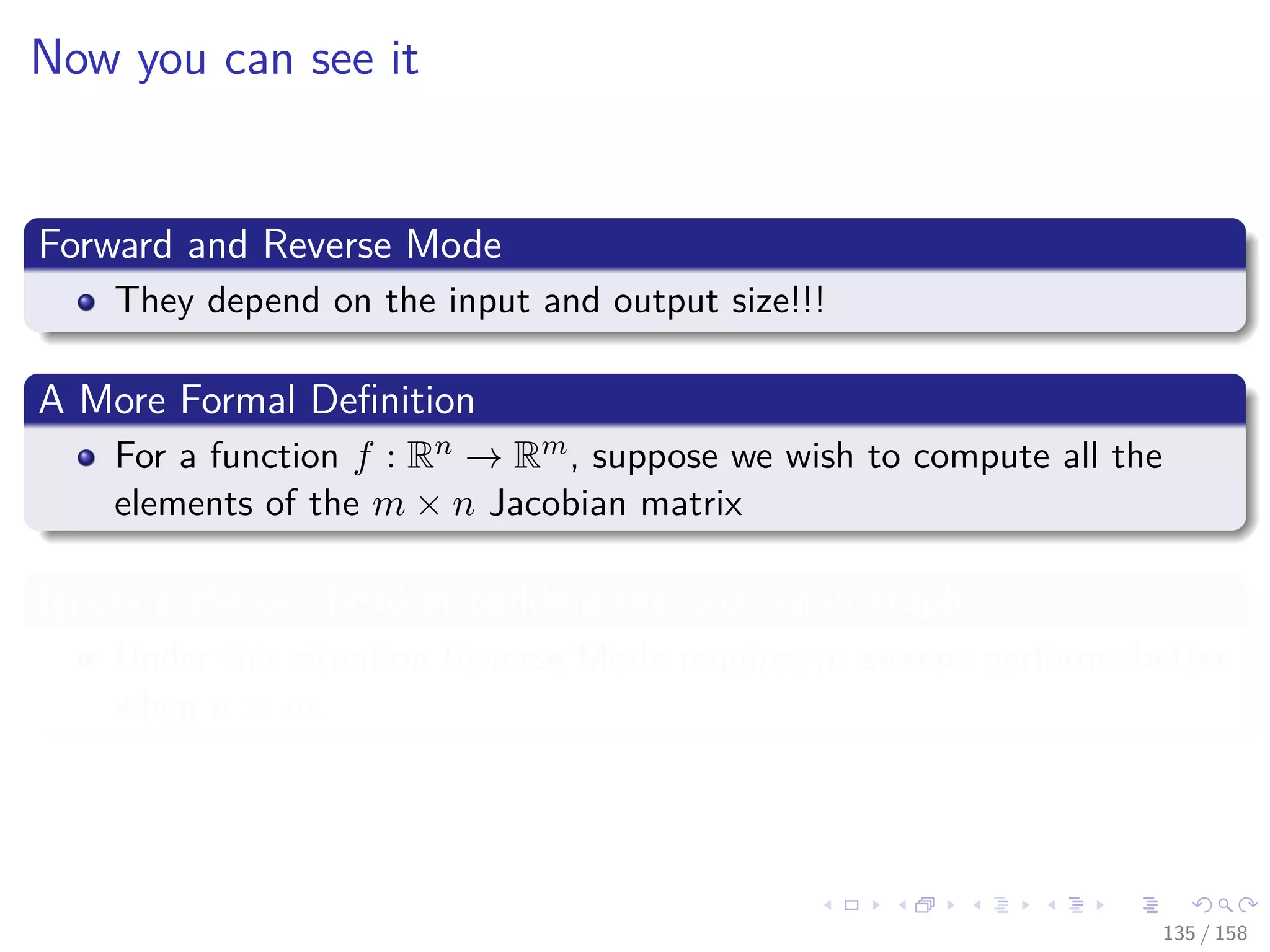
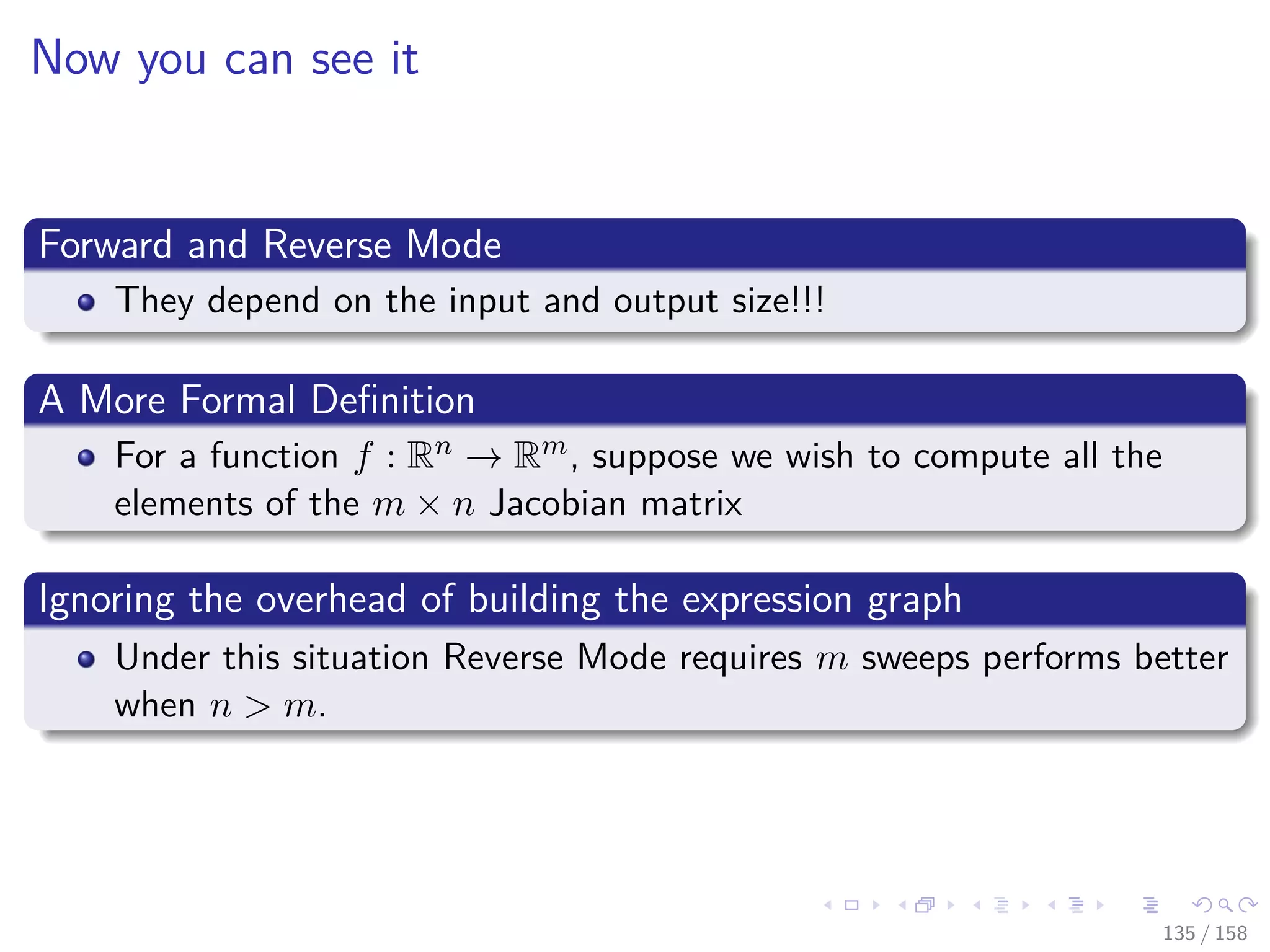
The problem of computing a full Jacobian of f : Rn
→ Rm
with a
minimum number of arithmetic operations
It is known as the Optimal Jacobian Accumulation (OJA) problem,
which is NP-complete [13].
154 / 158](https://image.slidesharecdn.com/05backpropagationautomaticdifferentiation-191105020025/75/05-backpropagation-automatic_differentiation-271-2048.jpg)
![Images/cinvestav
Between Two Extremes
Something Notable
Forward and reverse accumulation are just two (extreme) ways of
traversing the chain rule.
The problem of computing a full Jacobian of f : Rn
→ Rm
with a
minimum number of arithmetic operations
It is known as the Optimal Jacobian Accumulation (OJA) problem,
which is NP-complete [13].
154 / 158](https://image.slidesharecdn.com/05backpropagationautomaticdifferentiation-191105020025/75/05-backpropagation-automatic_differentiation-272-2048.jpg)
![Images/cinvestav
Finally
Using all the previous ideas
The Graph Structure Proposed in [2]
The Computational Graph of AD
The Forward and Reversal Methods
It has been possible to develop the Deep Learning Frameworks
TensorFlow
Torch
Pytorch
Keras
etc...
155 / 158](https://image.slidesharecdn.com/05backpropagationautomaticdifferentiation-191105020025/75/05-backpropagation-automatic_differentiation-273-2048.jpg)
![Images/cinvestav
Finally
Using all the previous ideas
The Graph Structure Proposed in [2]
The Computational Graph of AD
The Forward and Reversal Methods
It has been possible to develop the Deep Learning Frameworks
TensorFlow
Torch
Pytorch
Keras
etc...
155 / 158](https://image.slidesharecdn.com/05backpropagationautomaticdifferentiation-191105020025/75/05-backpropagation-automatic_differentiation-274-2048.jpg)

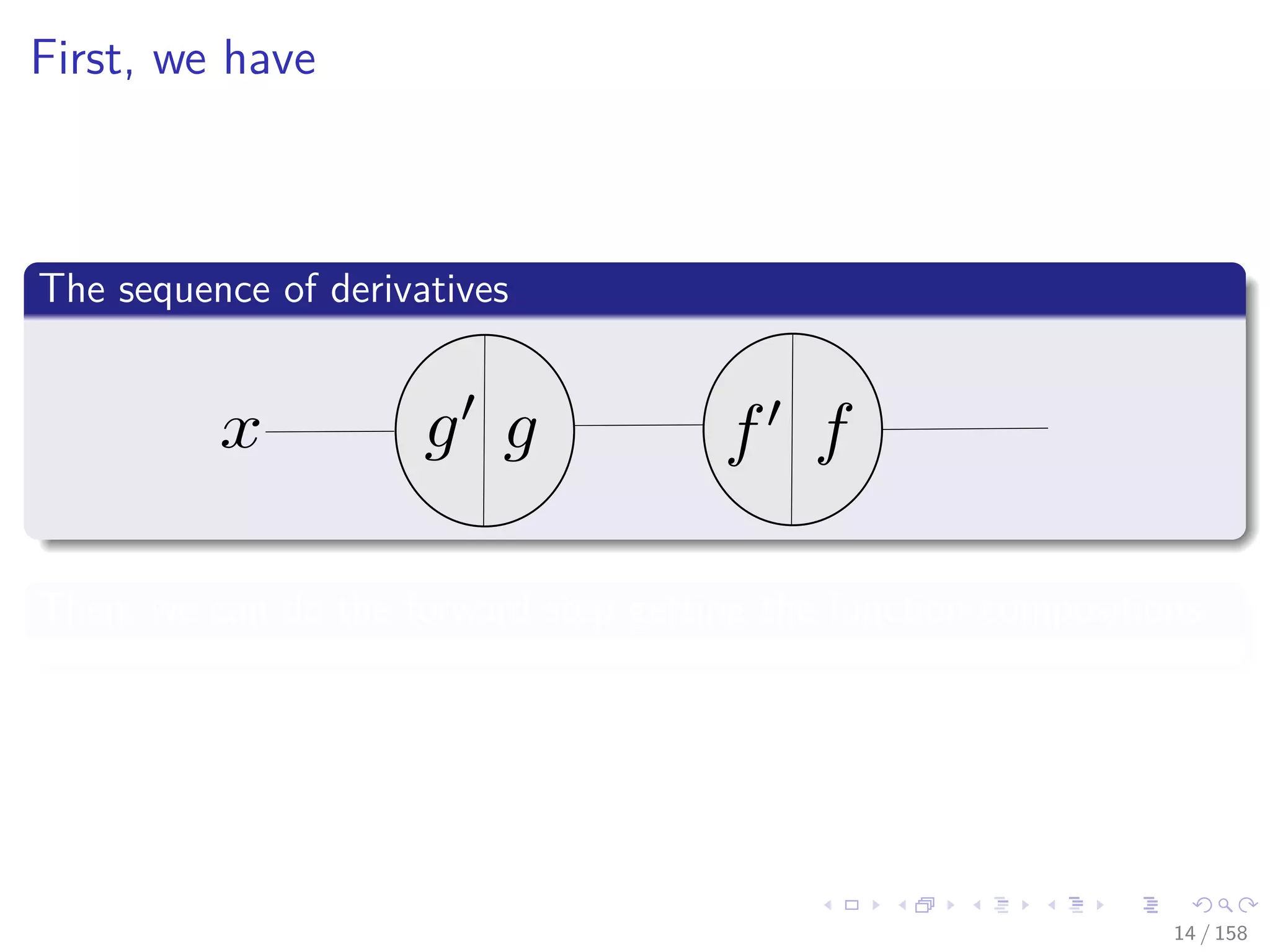
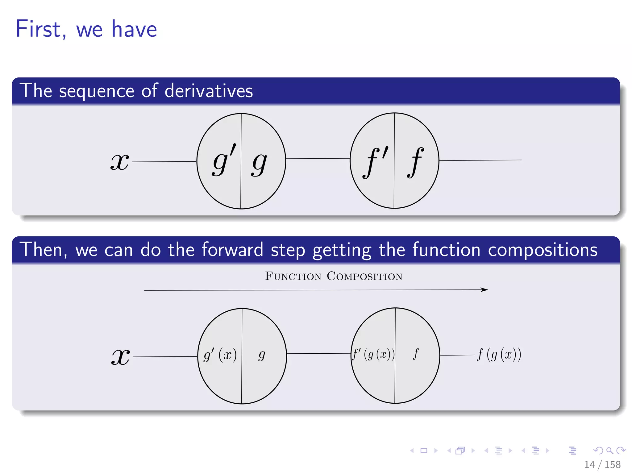
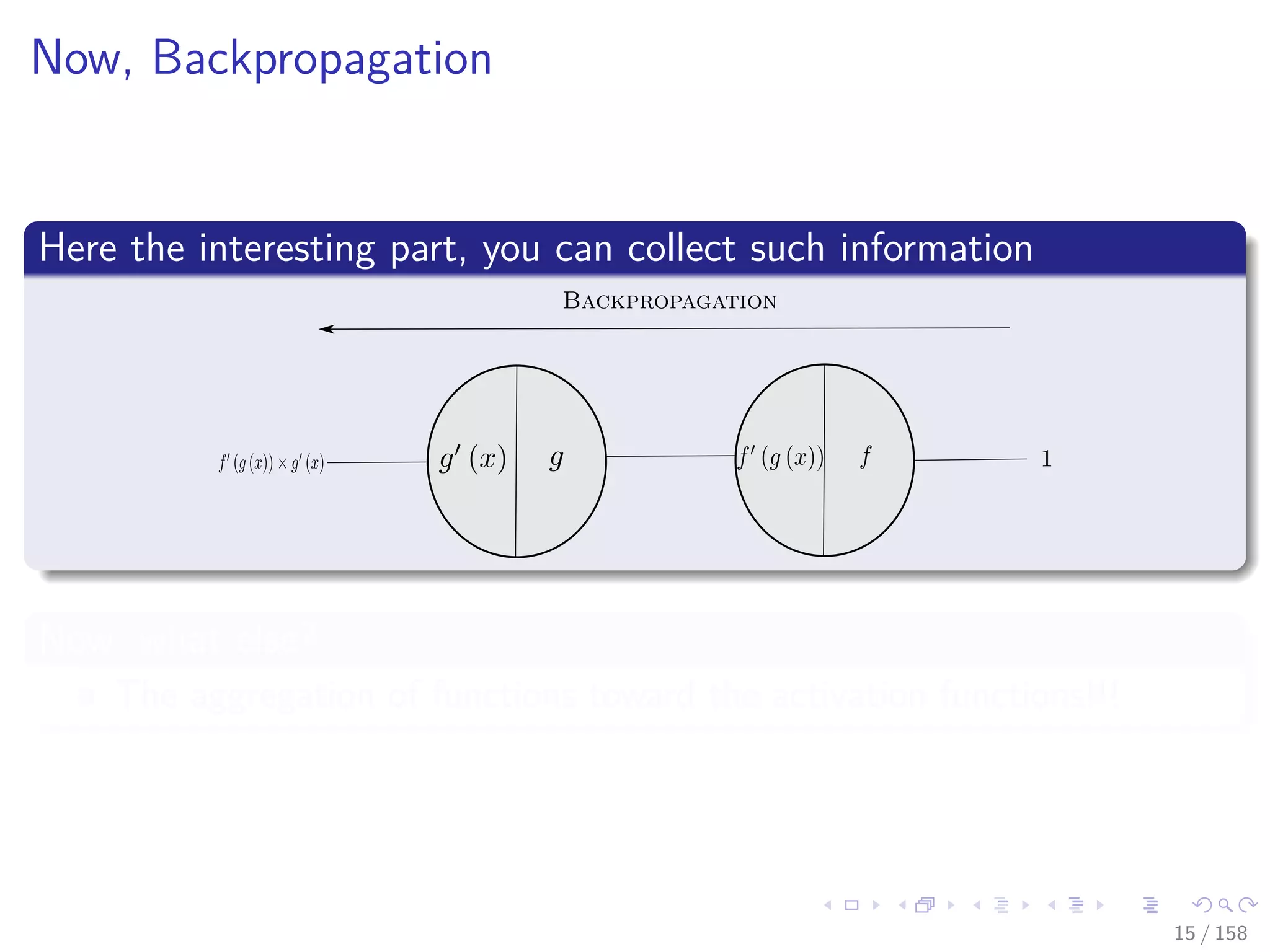
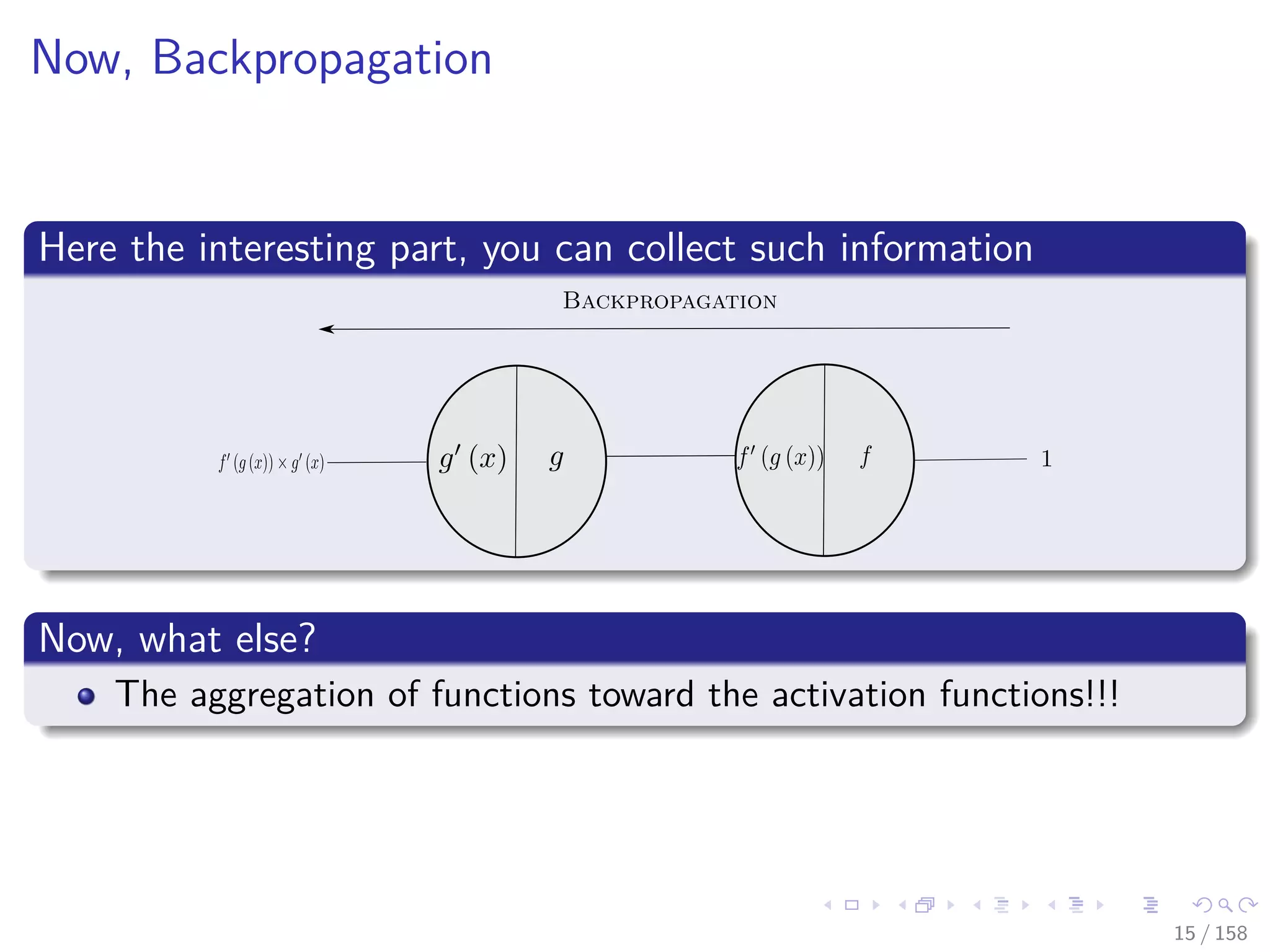
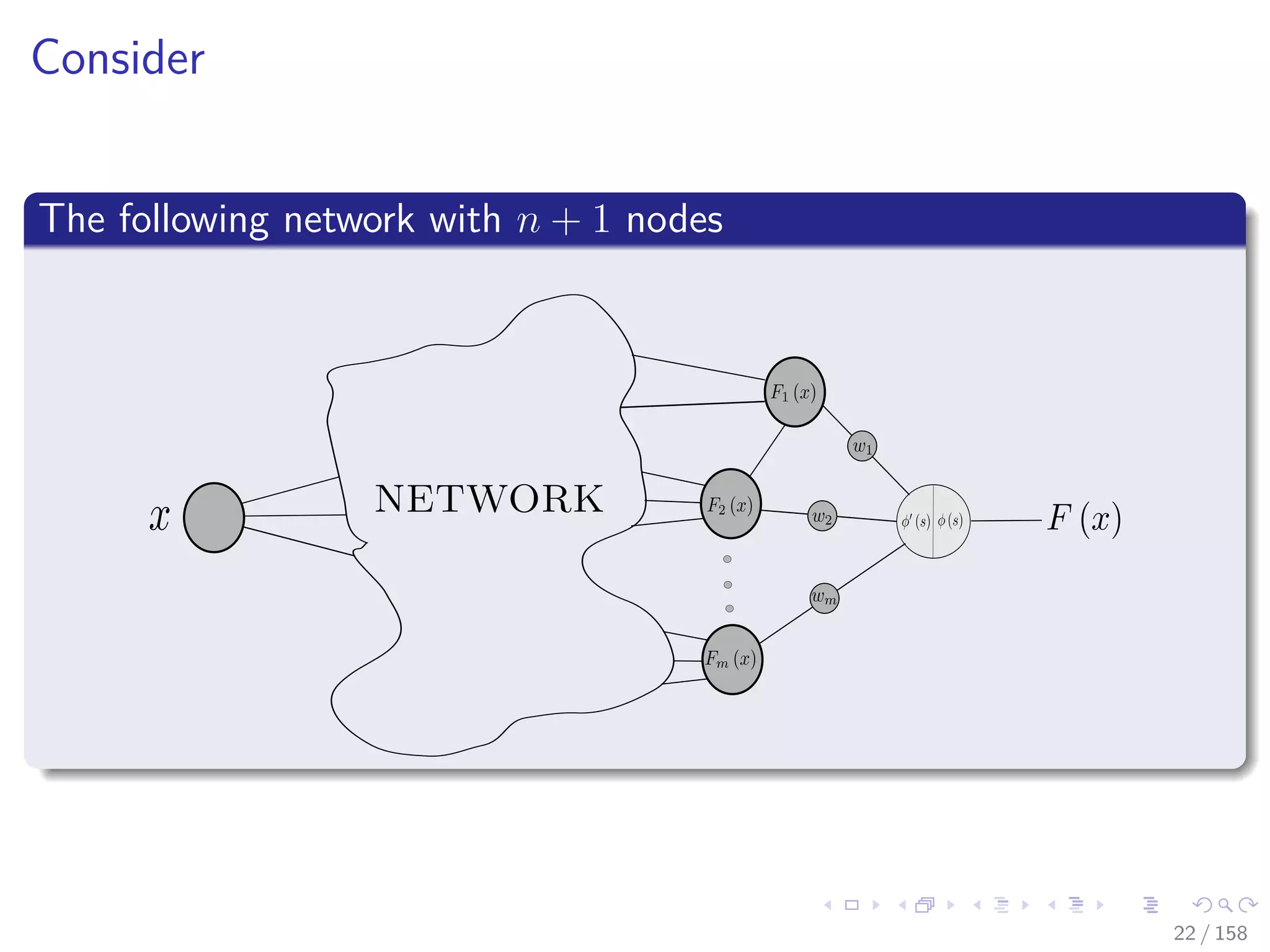
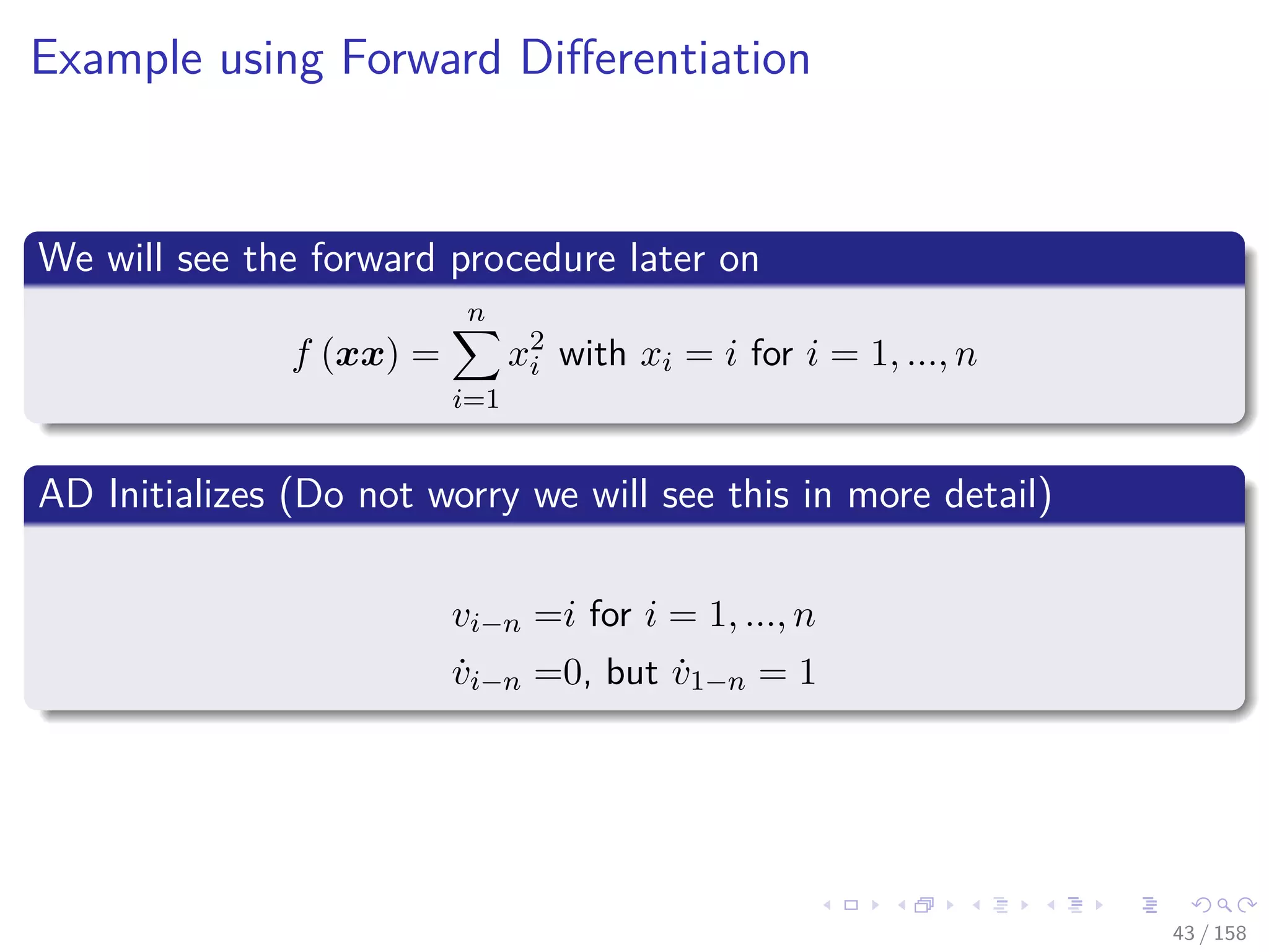
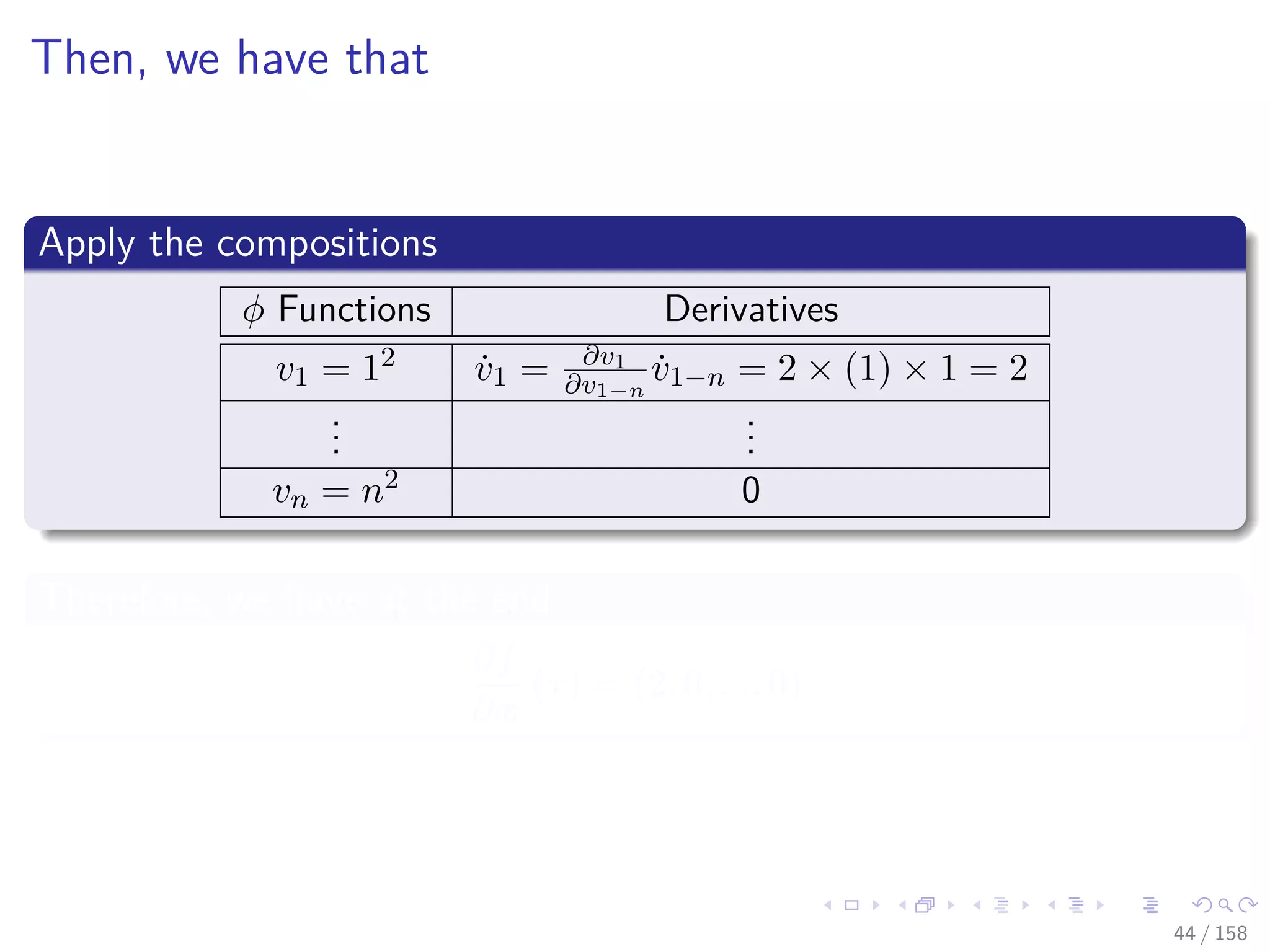
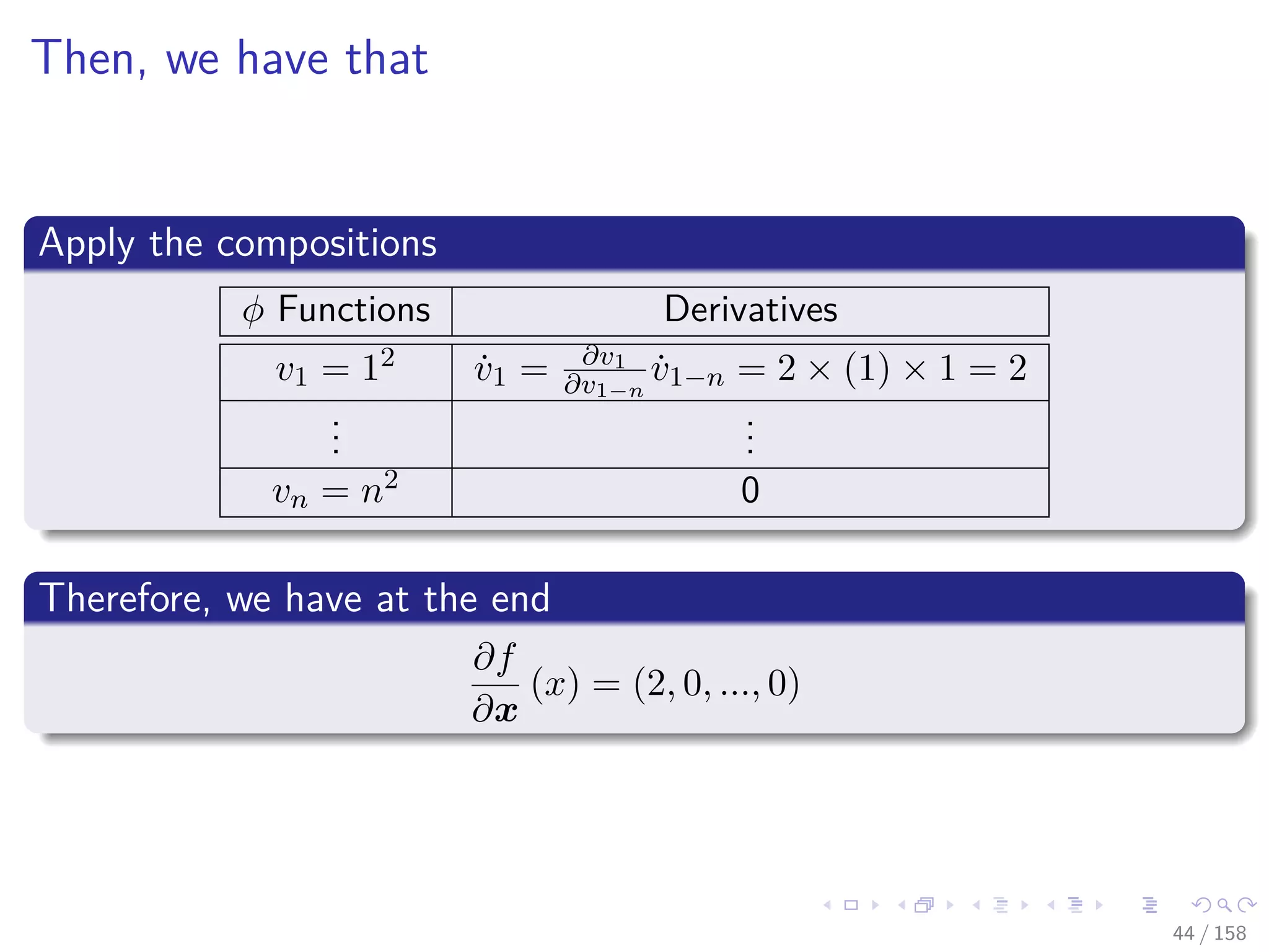
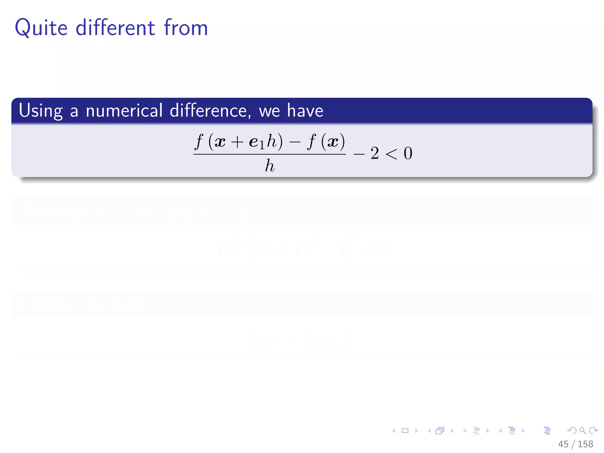
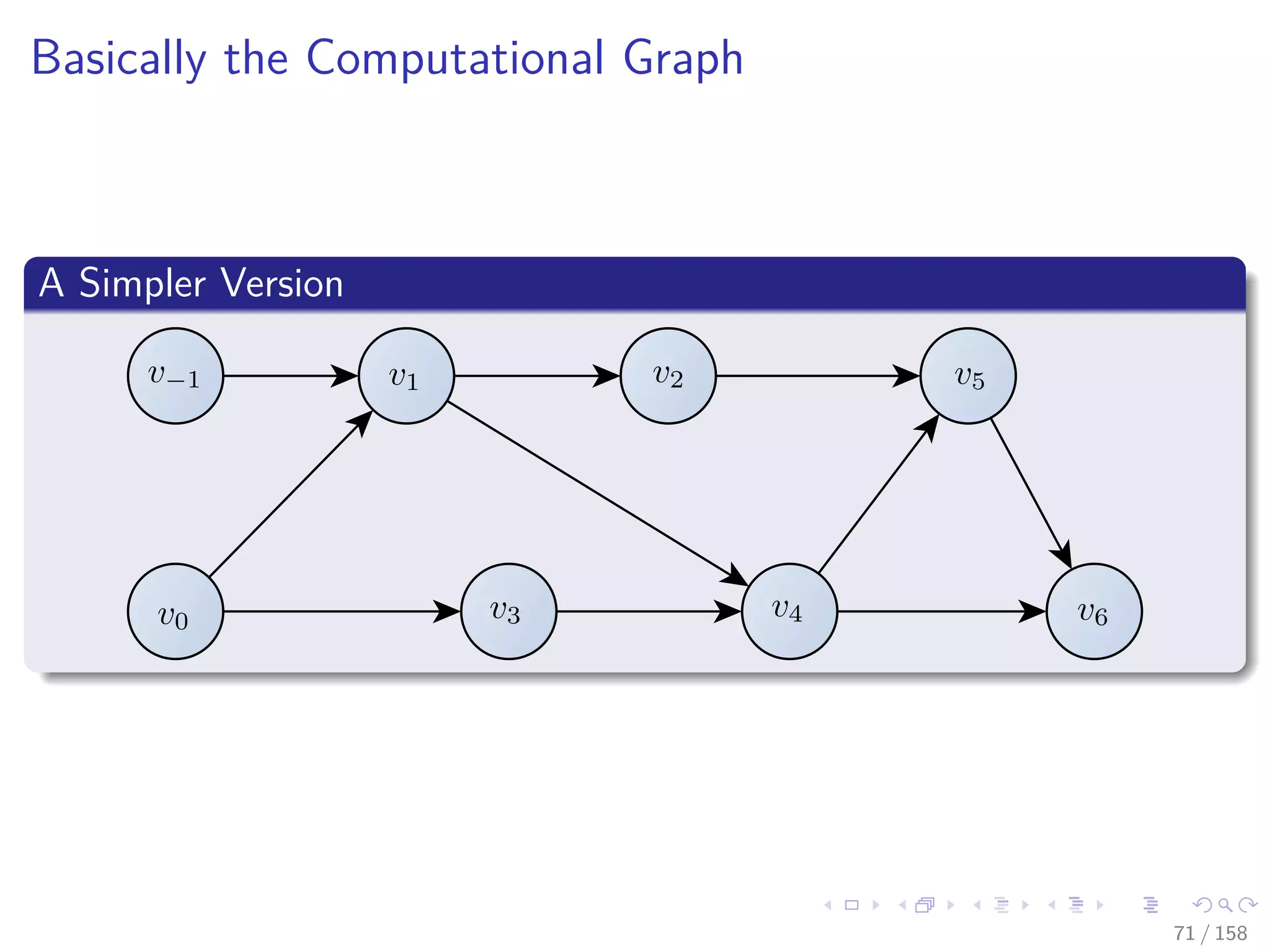
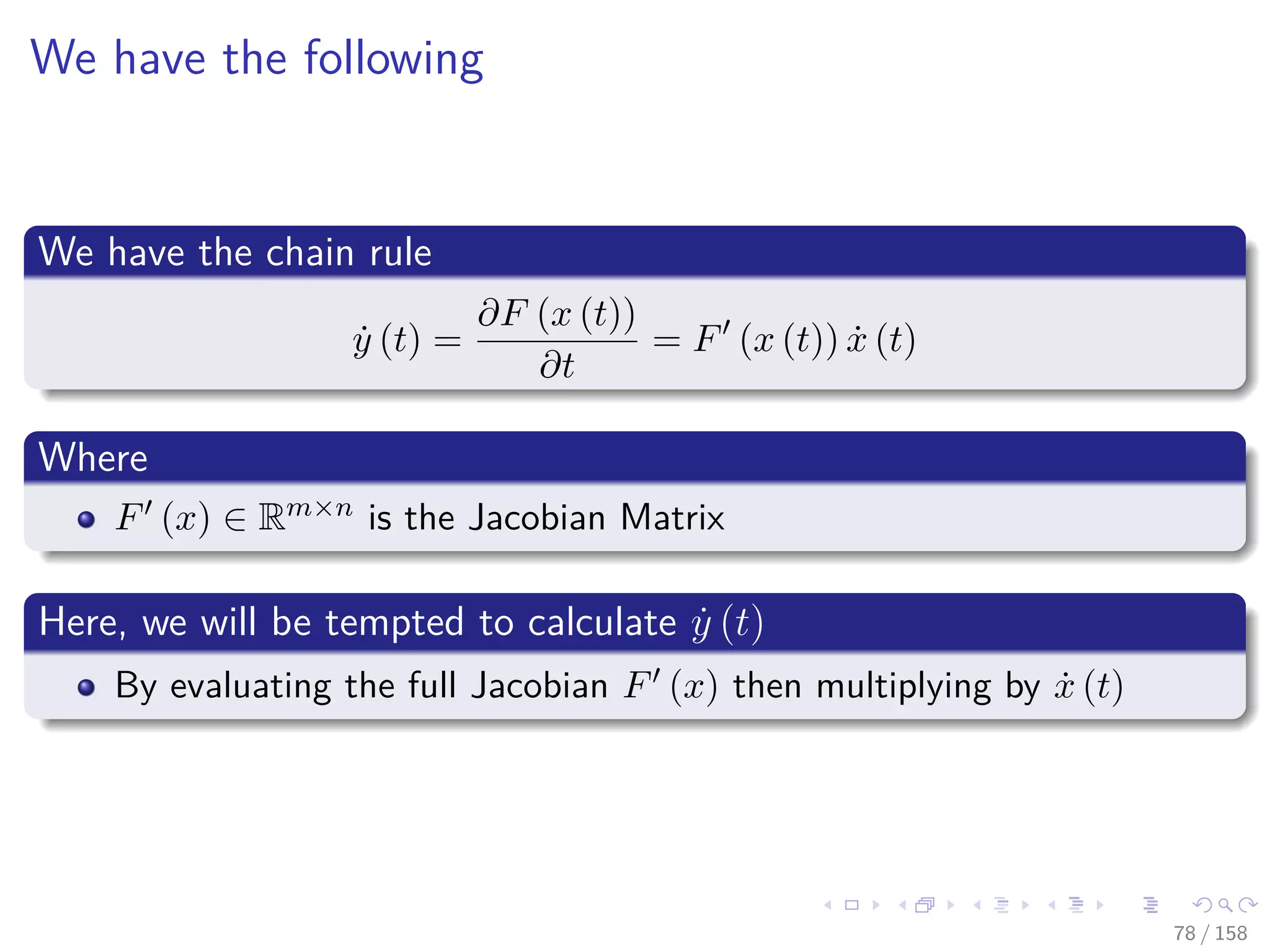
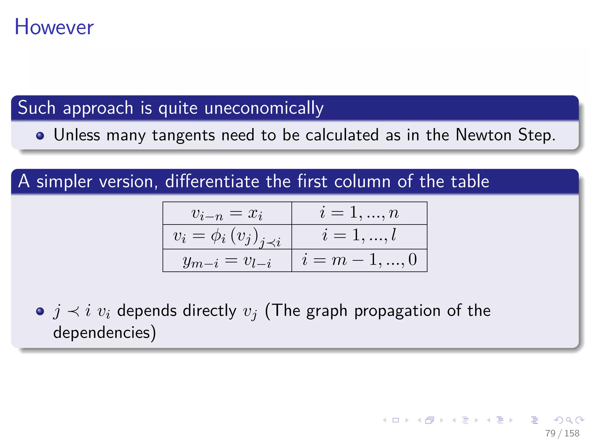
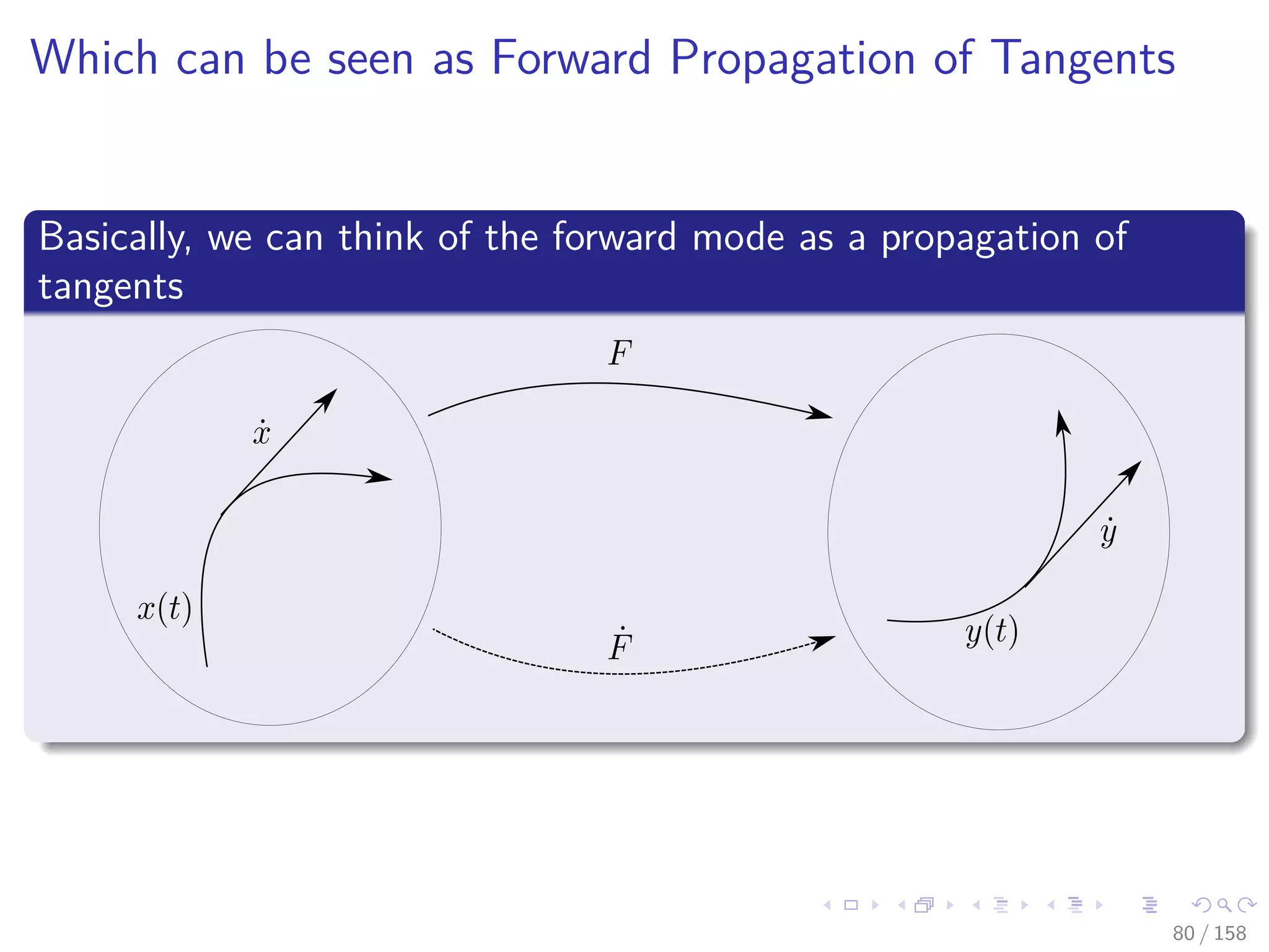
This document outlines and discusses backpropagation and automatic differentiation. It begins with an introduction to backpropagation, describing how it works in two phases: feed-forward to calculate outputs, and backpropagation to calculate gradients using the chain rule. It then discusses automatic differentiation, noting that it provides advantages over symbolic differentiation. The document explores the forward and reverse modes of automatic differentiation and examines their implementation and complexity. In summary, it covers the fundamental algorithms and methods for calculating gradients in neural networks.