Download as PDF, PPTX


![Therefore
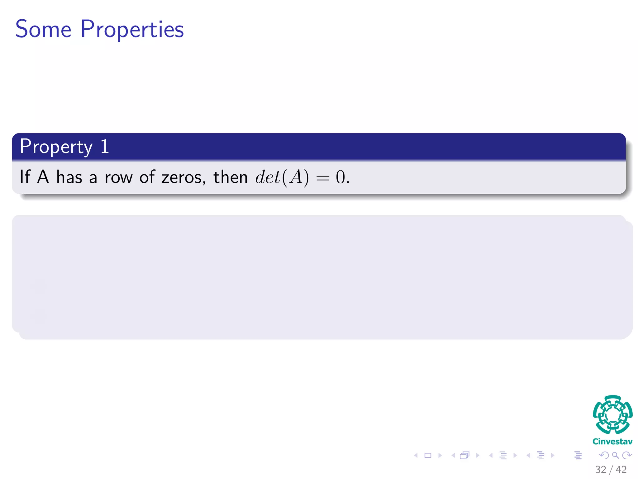
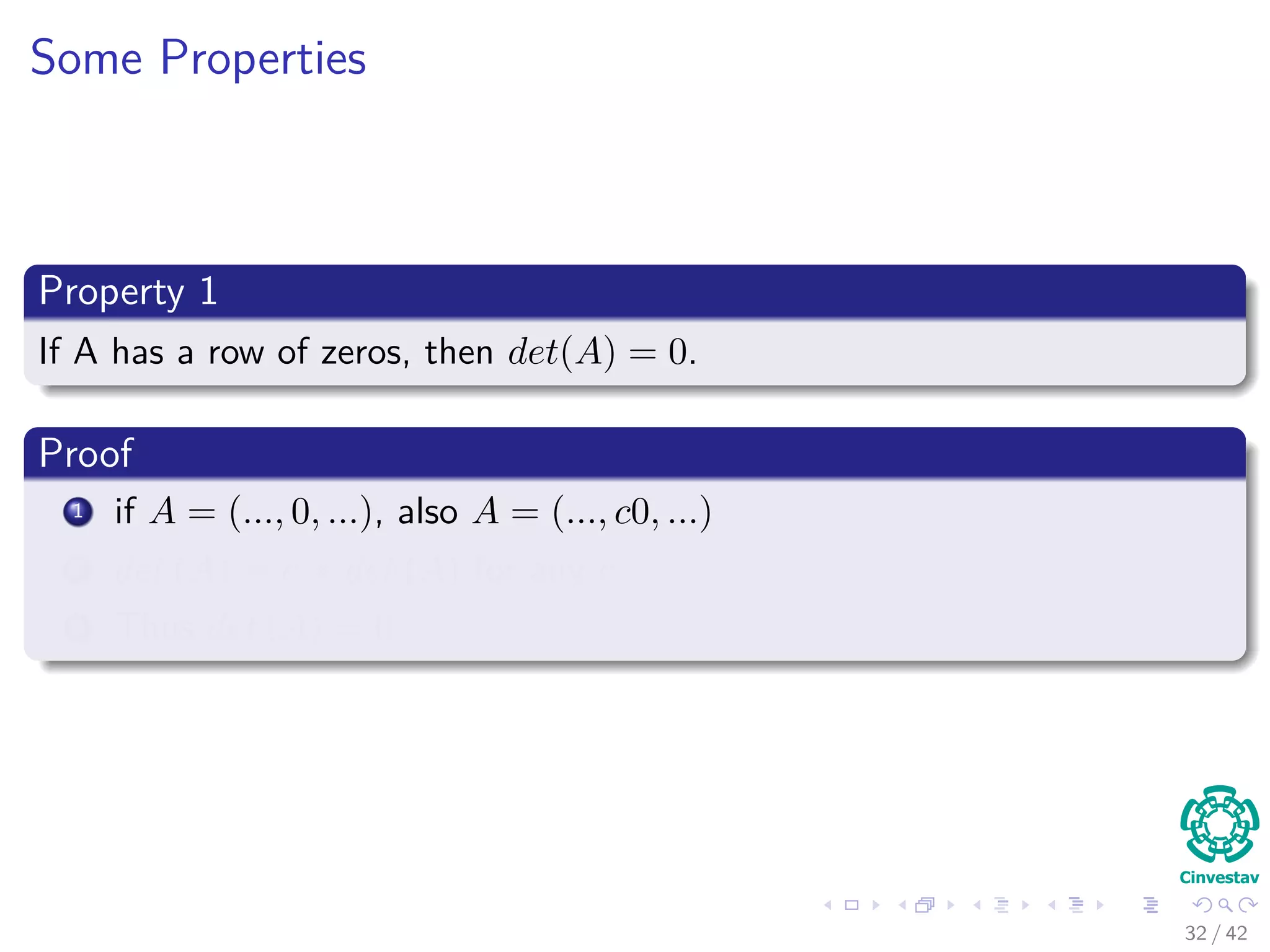
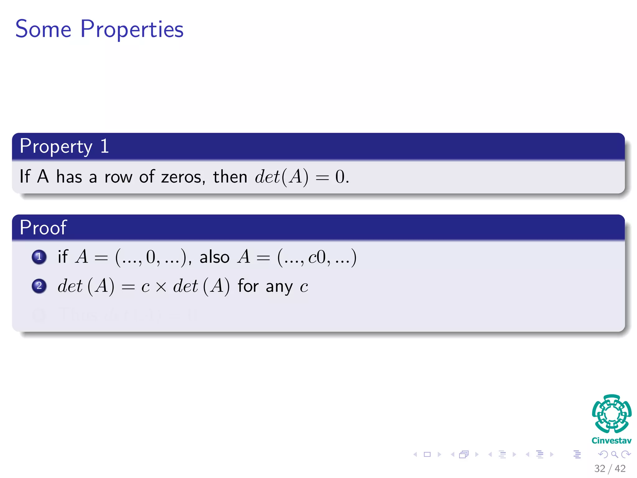
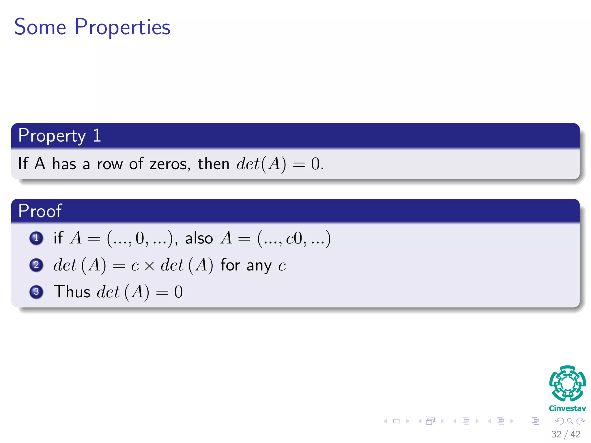
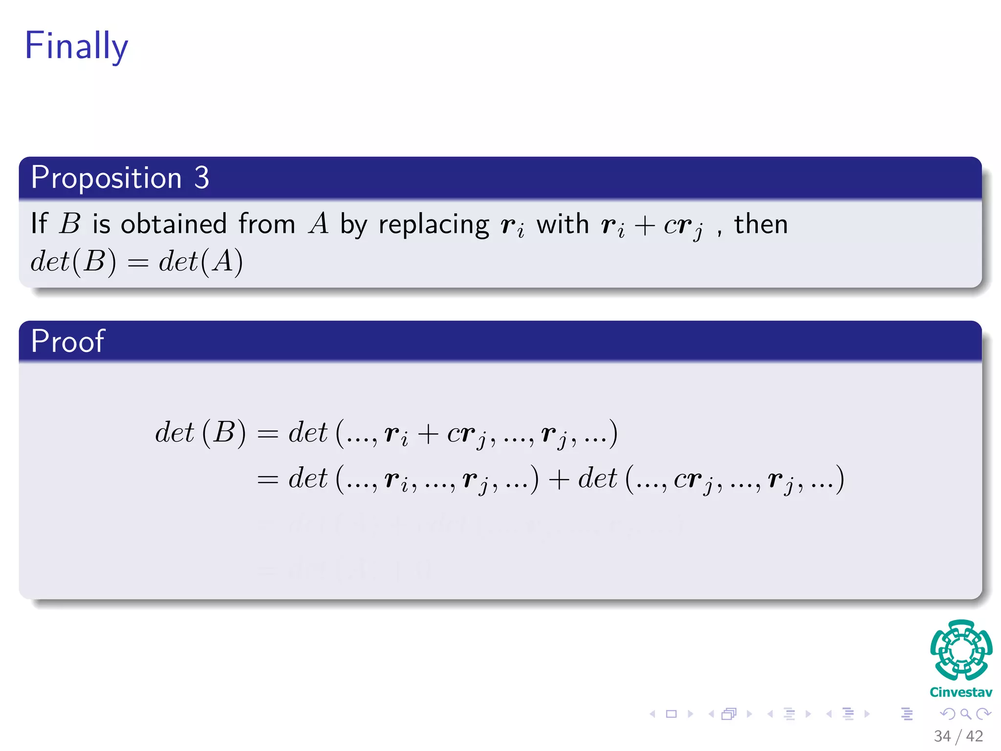
Theorem
The determinant of an upper or lower triangular matrix is equal to the
product of the entries on the main diagonal.
Proof
Suppose A is upper triangular and that none of the entries on the
main diagonal is 0.
This means all the entries beneath the main diagonal are zero.
Using Proposition 3, we can convert it into a diagonal matrix.
Then, by property 1
det (Adiag) = [
n
i aii] det (I) =
n
i aii
36 / 42](https://image.slidesharecdn.com/01-200420204445/75/01-03-squared-matrices_and_other_issues-79-2048.jpg)
![Therefore
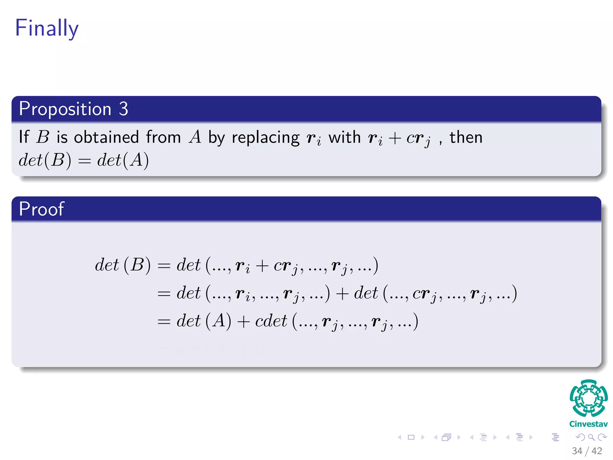
Theorem
The determinant of an upper or lower triangular matrix is equal to the
product of the entries on the main diagonal.
Proof
Suppose A is upper triangular and that none of the entries on the
main diagonal is 0.
This means all the entries beneath the main diagonal are zero.
Using Proposition 3, we can convert it into a diagonal matrix.
Then, by property 1
det (Adiag) = [
n
i aii] det (I) =
n
i aii
36 / 42](https://image.slidesharecdn.com/01-200420204445/75/01-03-squared-matrices_and_other_issues-80-2048.jpg)
![Therefore
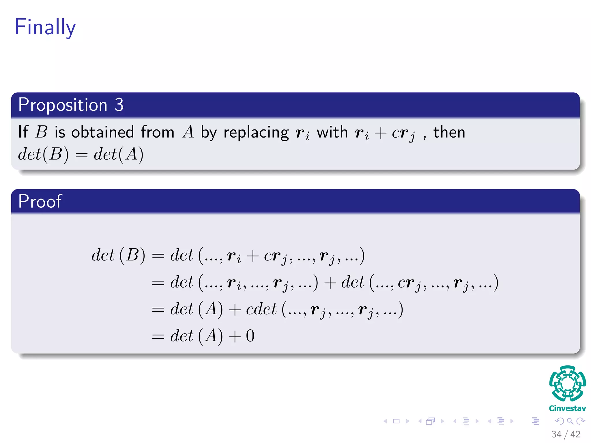
Theorem
The determinant of an upper or lower triangular matrix is equal to the
product of the entries on the main diagonal.
Proof
Suppose A is upper triangular and that none of the entries on the
main diagonal is 0.
This means all the entries beneath the main diagonal are zero.
Using Proposition 3, we can convert it into a diagonal matrix.
Then, by property 1
det (Adiag) = [
n
i aii] det (I) =
n
i aii
36 / 42](https://image.slidesharecdn.com/01-200420204445/75/01-03-squared-matrices_and_other_issues-81-2048.jpg)
![Therefore
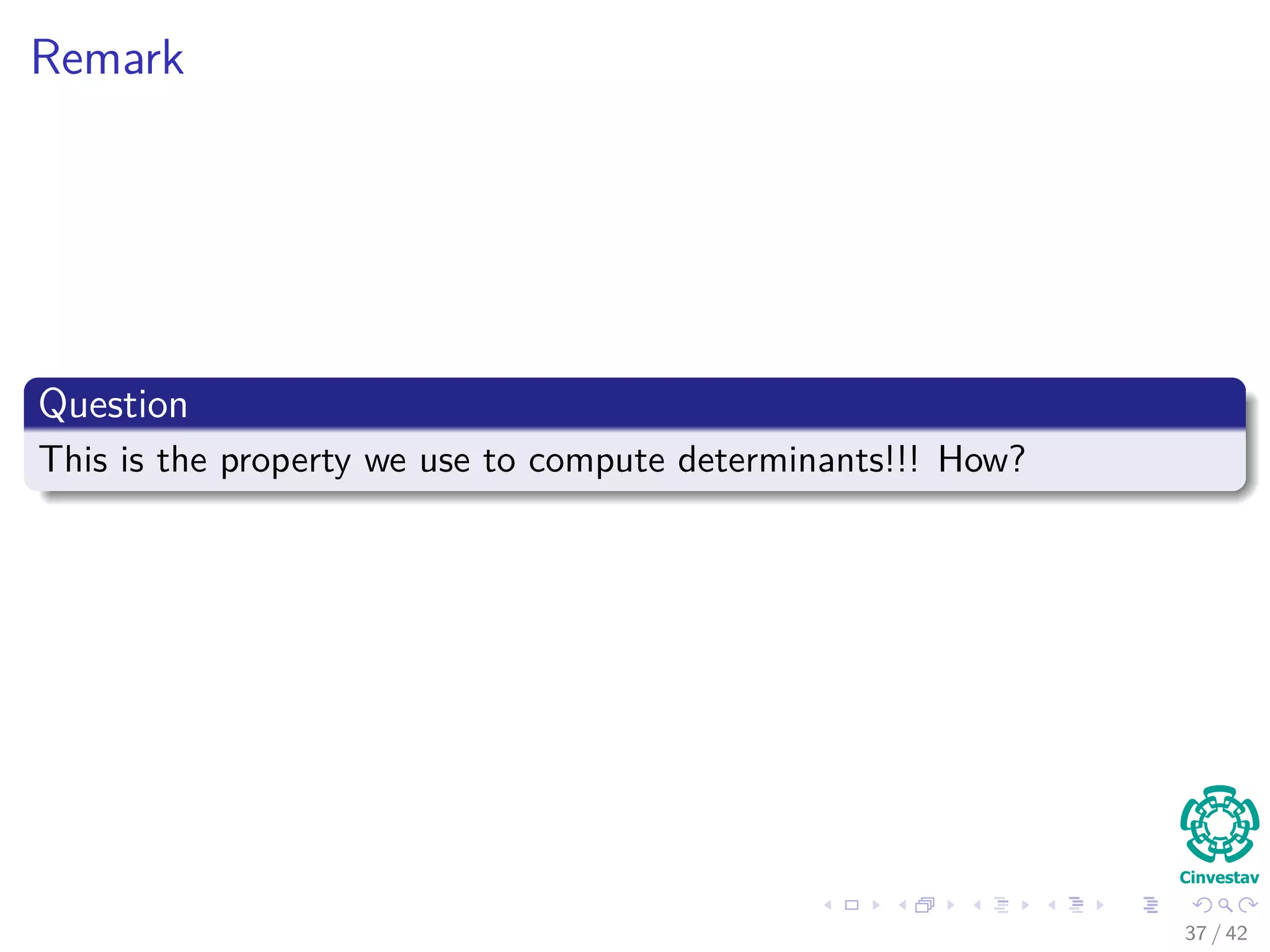
Theorem
The determinant of an upper or lower triangular matrix is equal to the
product of the entries on the main diagonal.
Proof
Suppose A is upper triangular and that none of the entries on the
main diagonal is 0.
This means all the entries beneath the main diagonal are zero.
Using Proposition 3, we can convert it into a diagonal matrix.
Then, by property 1
det (Adiag) = [
n
i aii] det (I) =
n
i aii
36 / 42](https://image.slidesharecdn.com/01-200420204445/75/01-03-squared-matrices_and_other_issues-82-2048.jpg)
![Therefore
Theorem
The determinant of an upper or lower triangular matrix is equal to the
product of the entries on the main diagonal.
Proof
Suppose A is upper triangular and that none of the entries on the
main diagonal is 0.
This means all the entries beneath the main diagonal are zero.
Using Proposition 3, we can convert it into a diagonal matrix.
Then, by property 1
det (Adiag) = [
n
i aii] det (I) =
n
i aii
36 / 42](https://image.slidesharecdn.com/01-200420204445/75/01-03-squared-matrices_and_other_issues-83-2048.jpg)
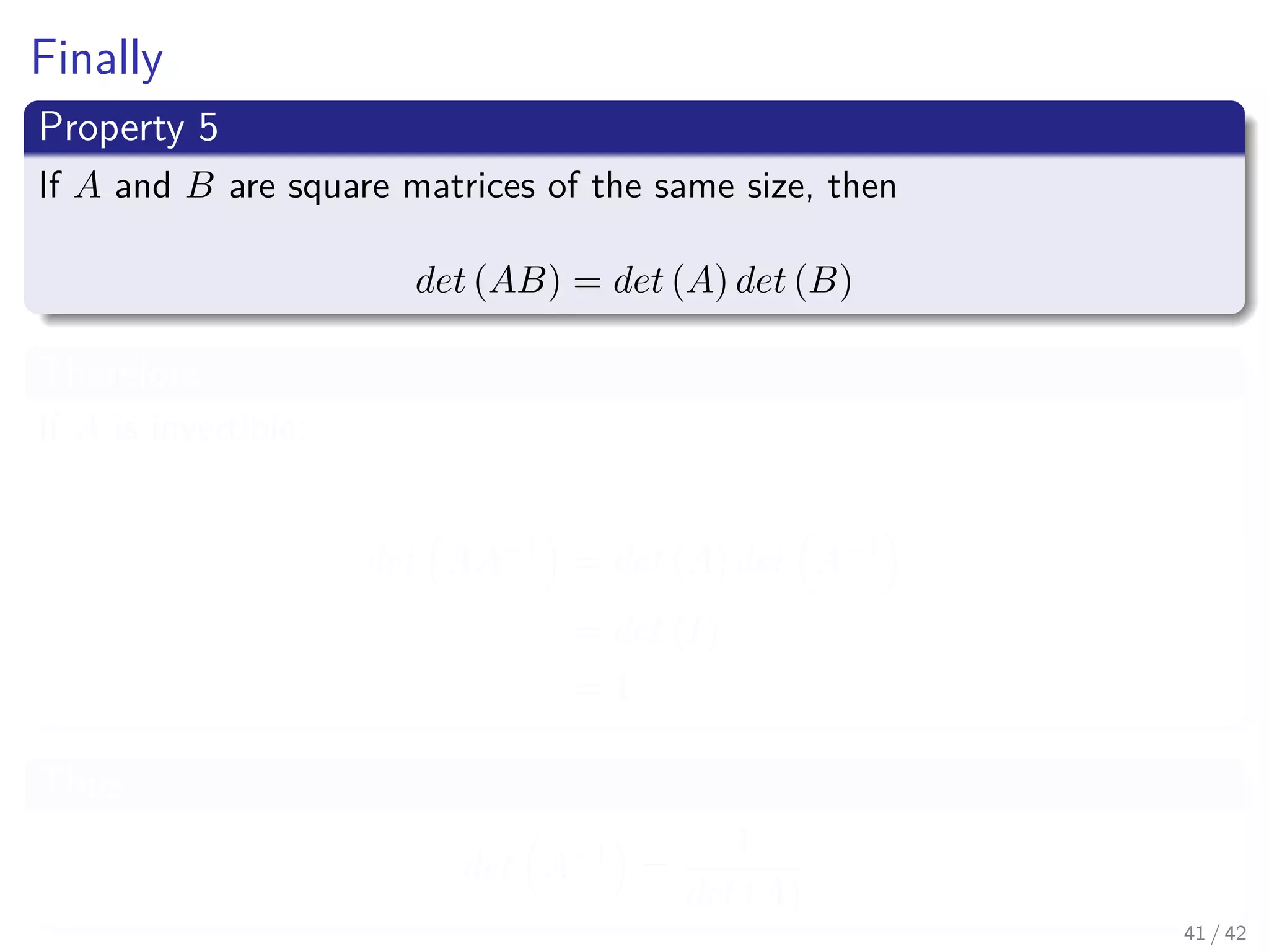
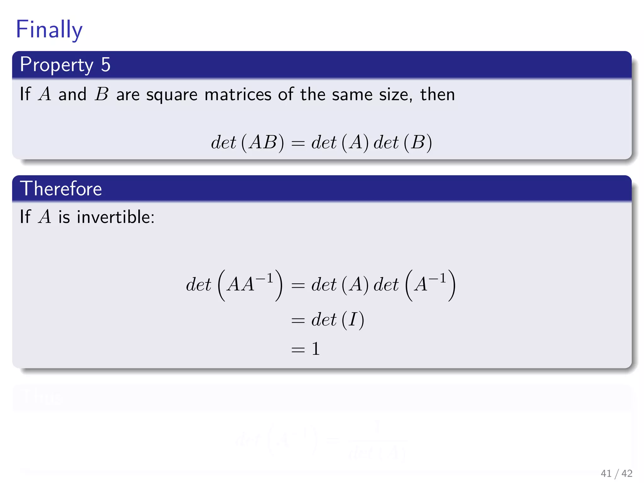
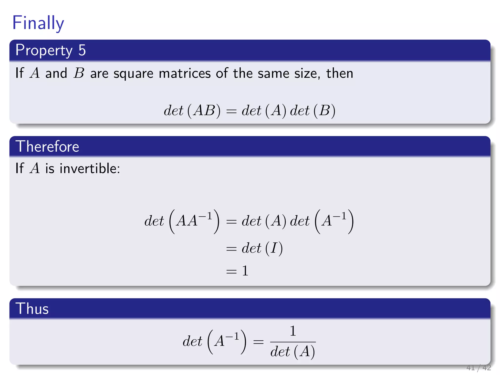
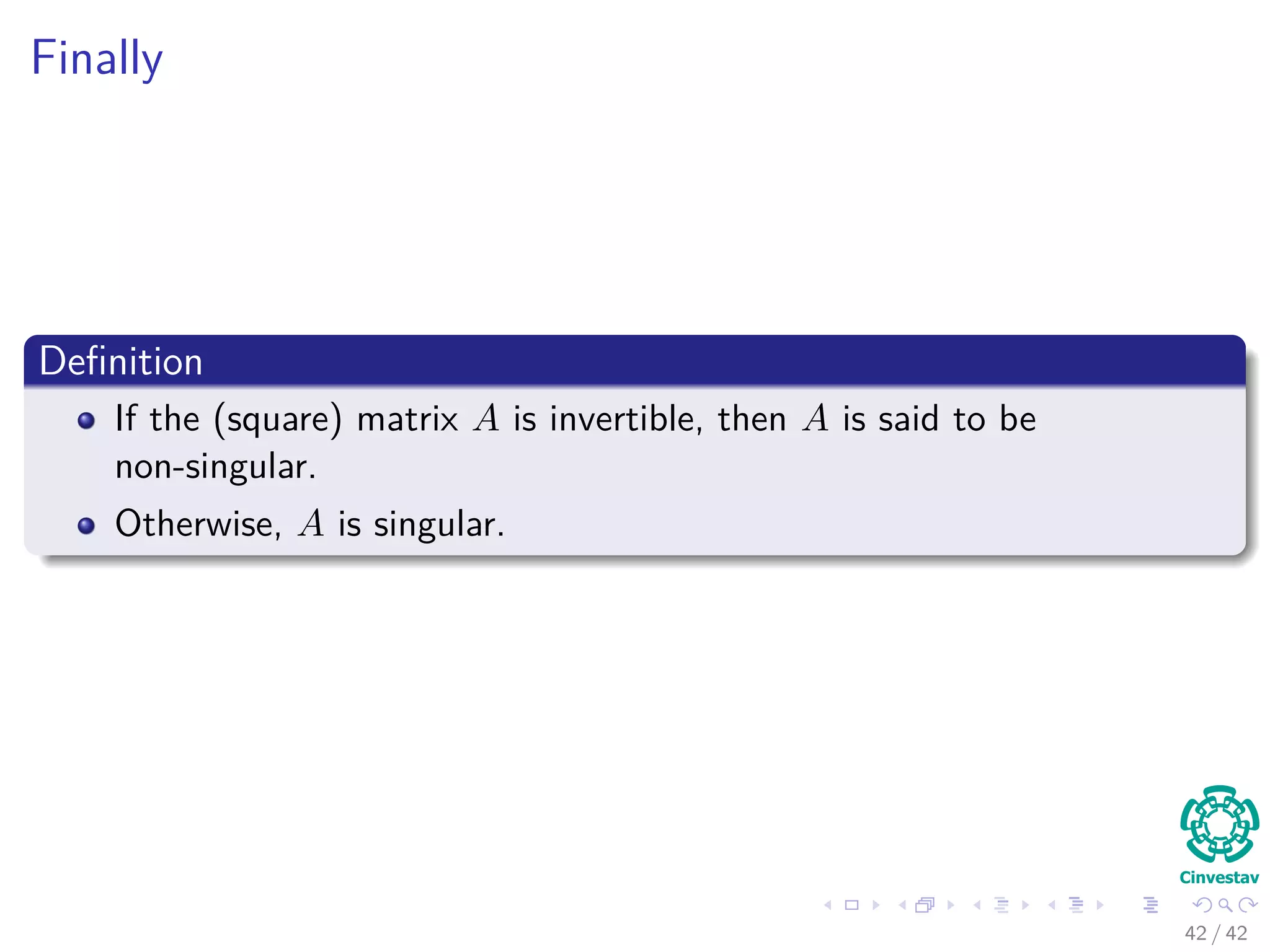

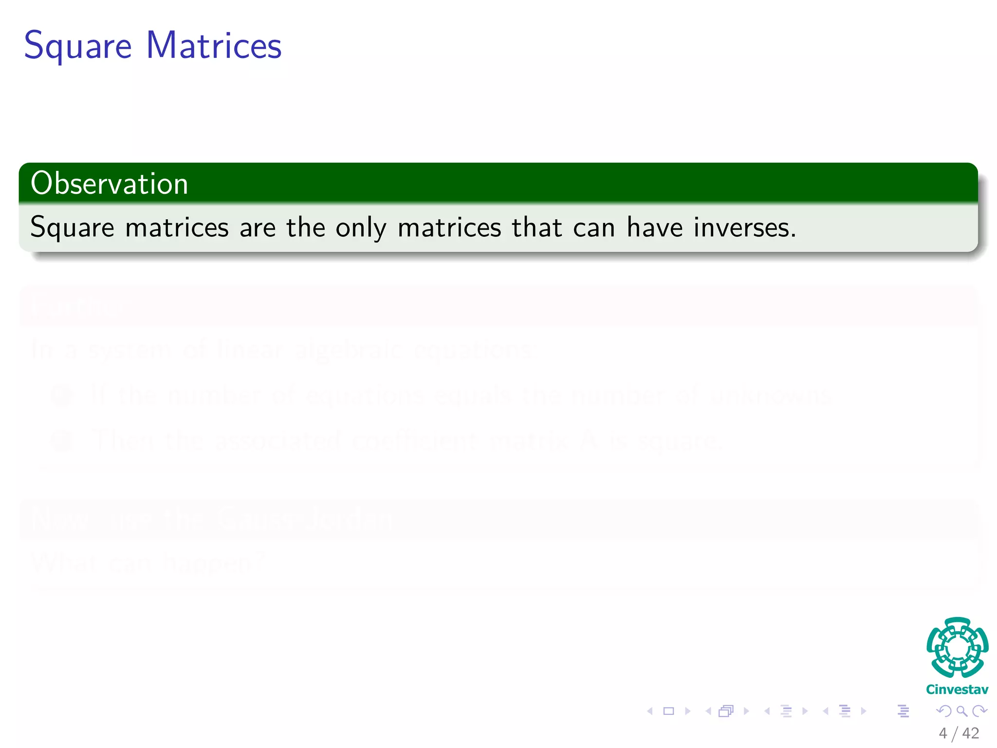
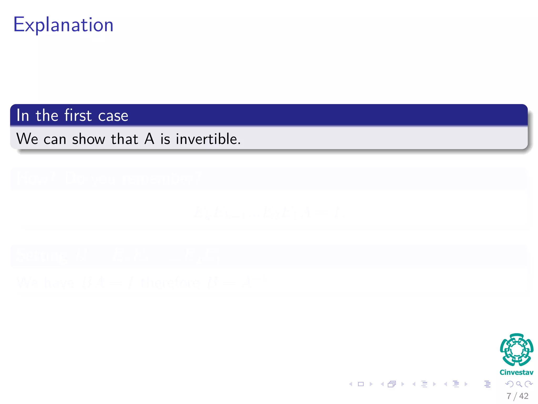
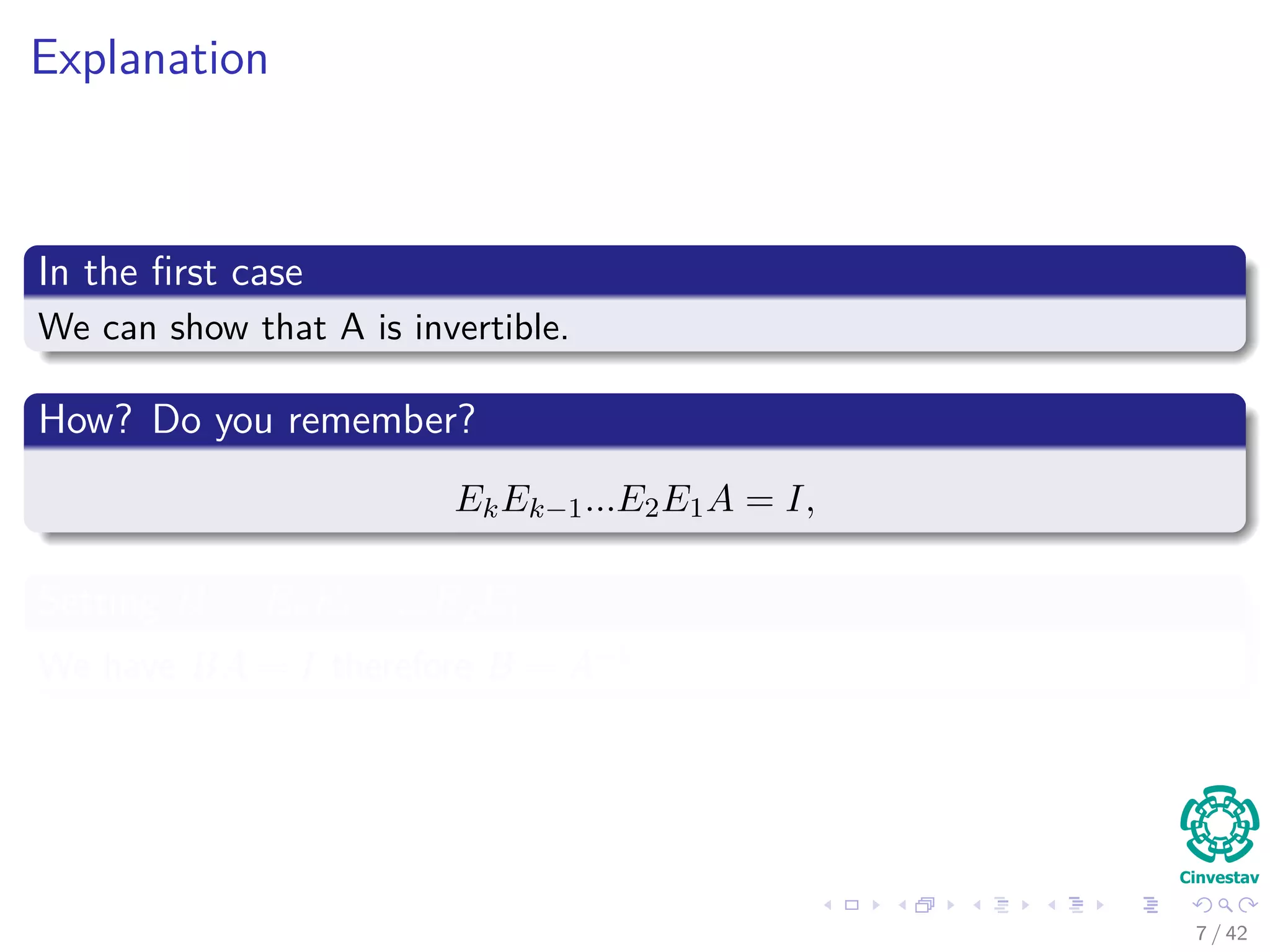
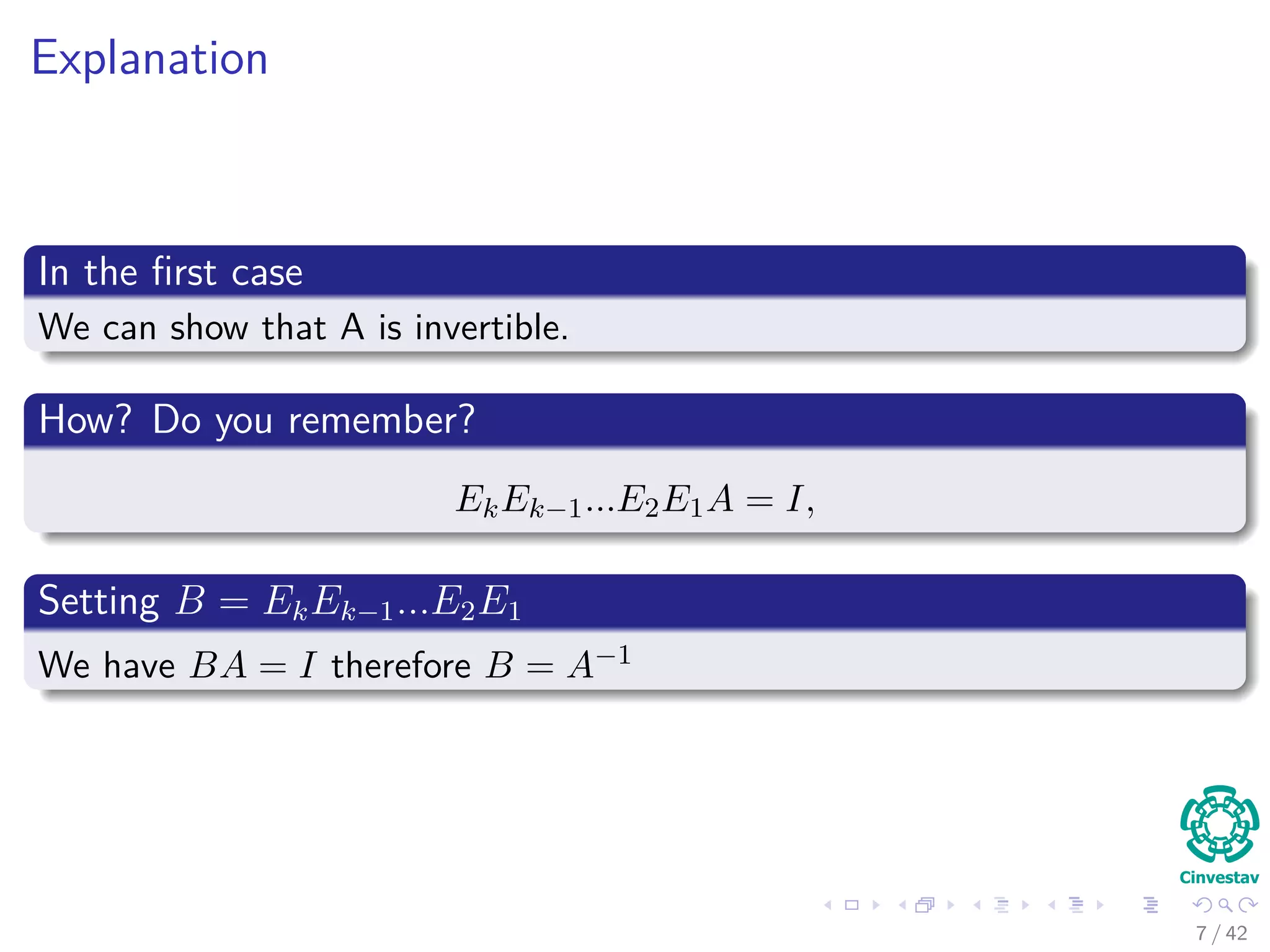
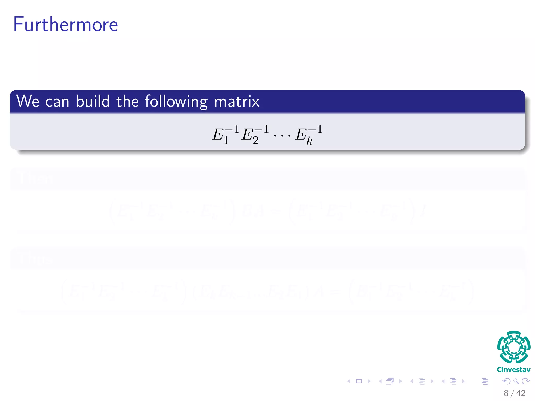
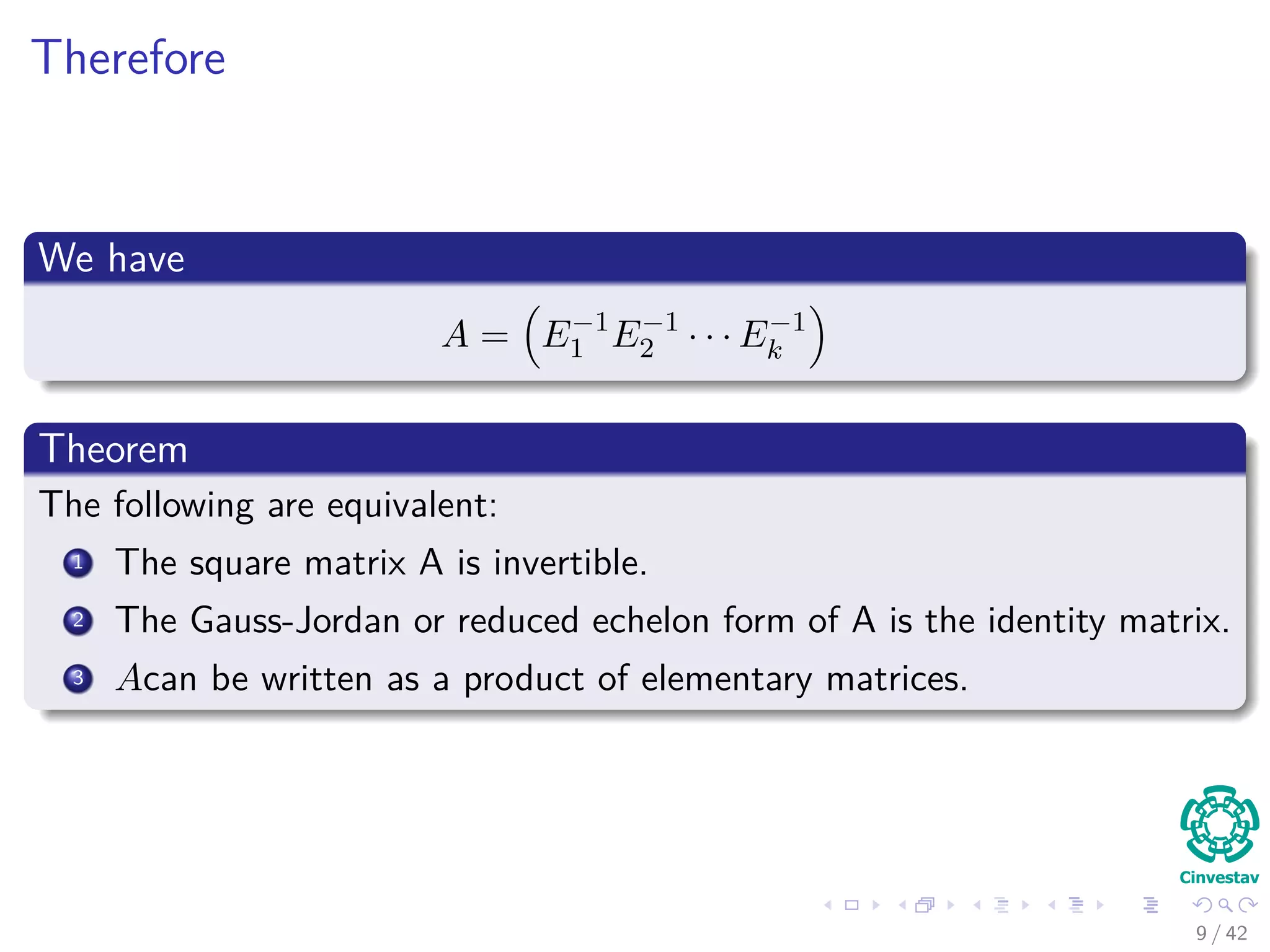
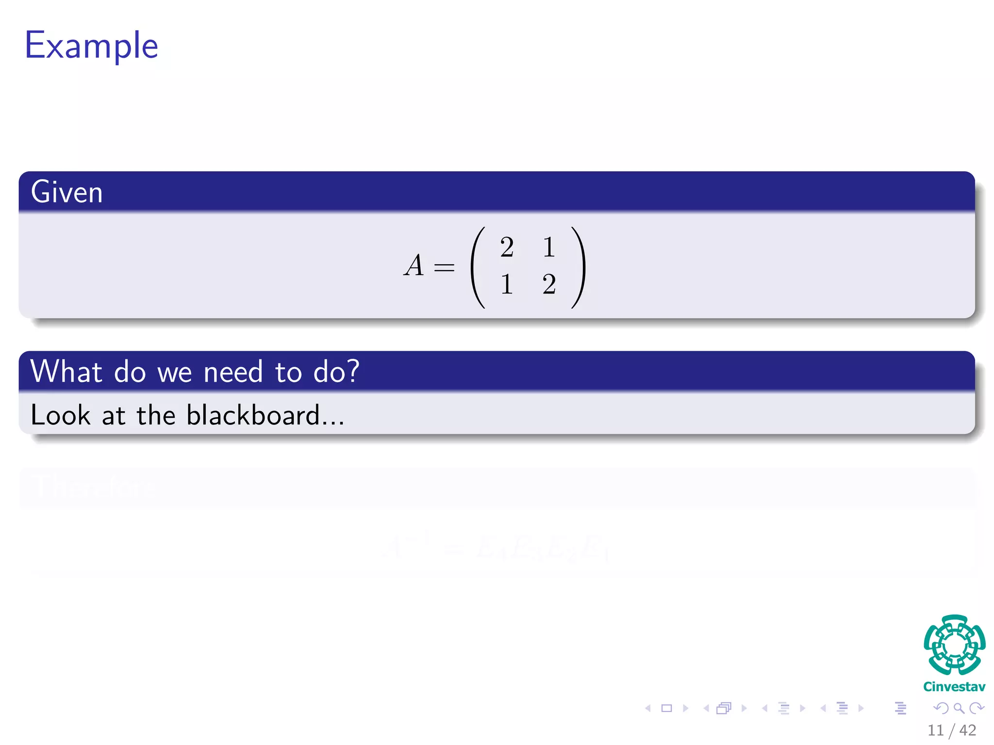
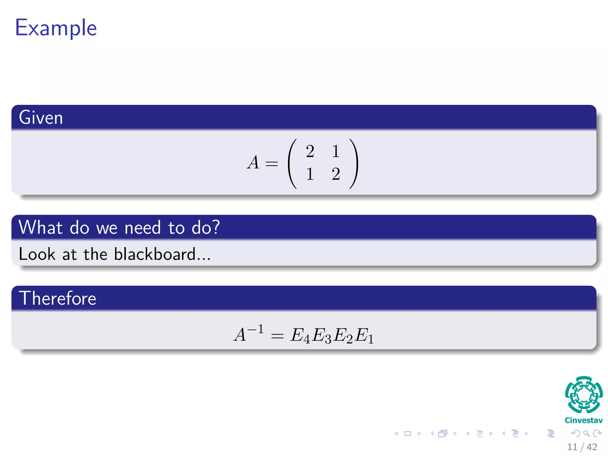
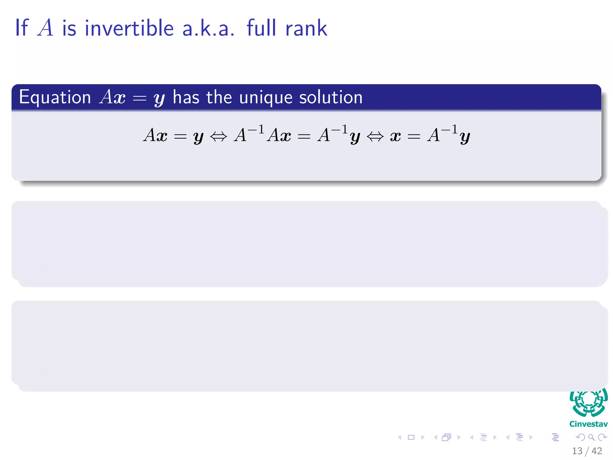
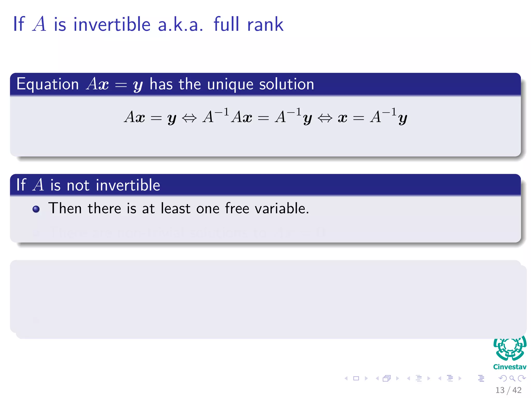
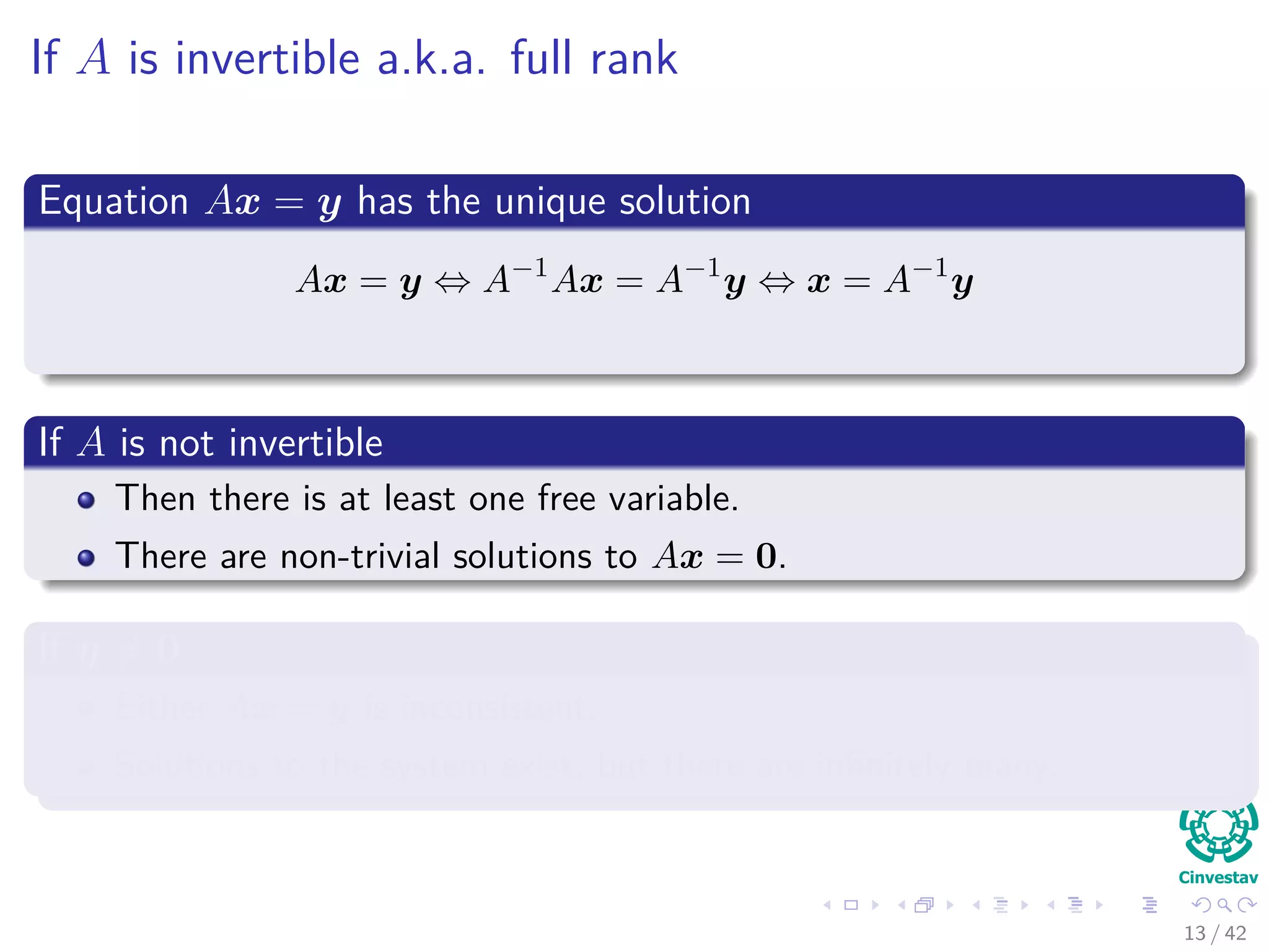
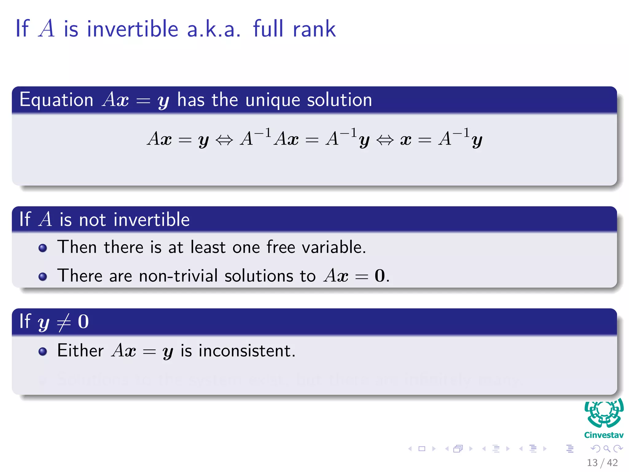
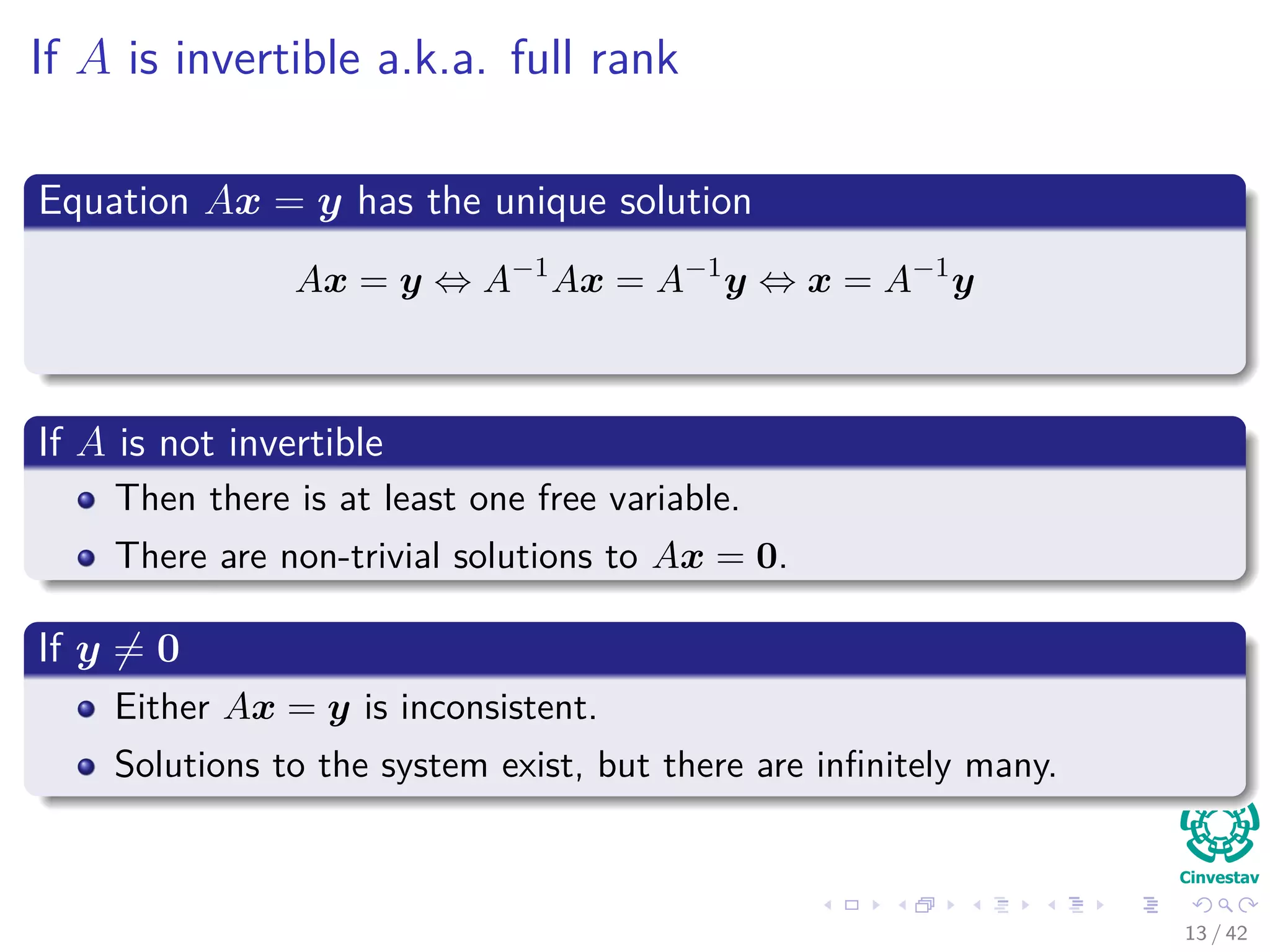
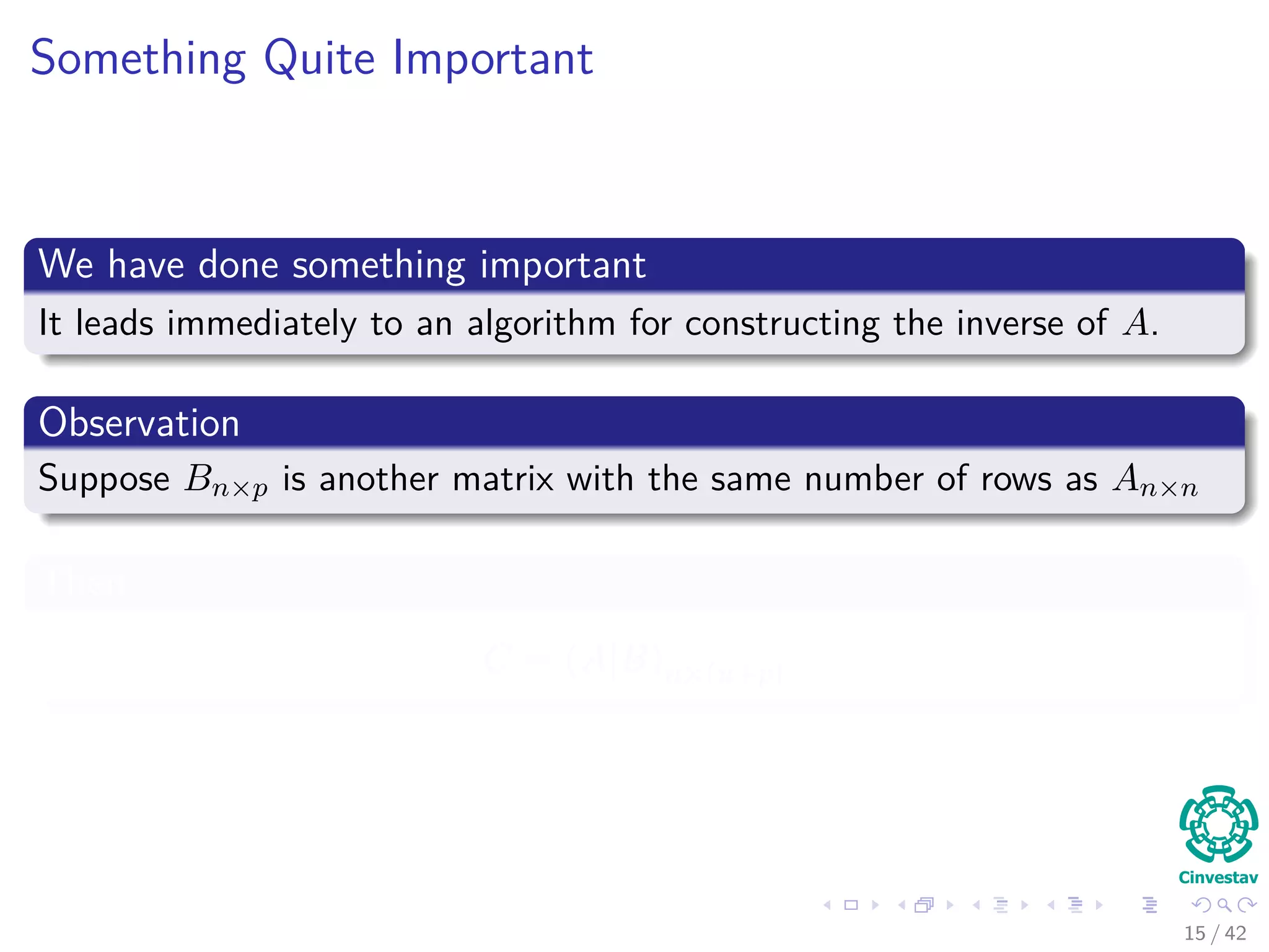
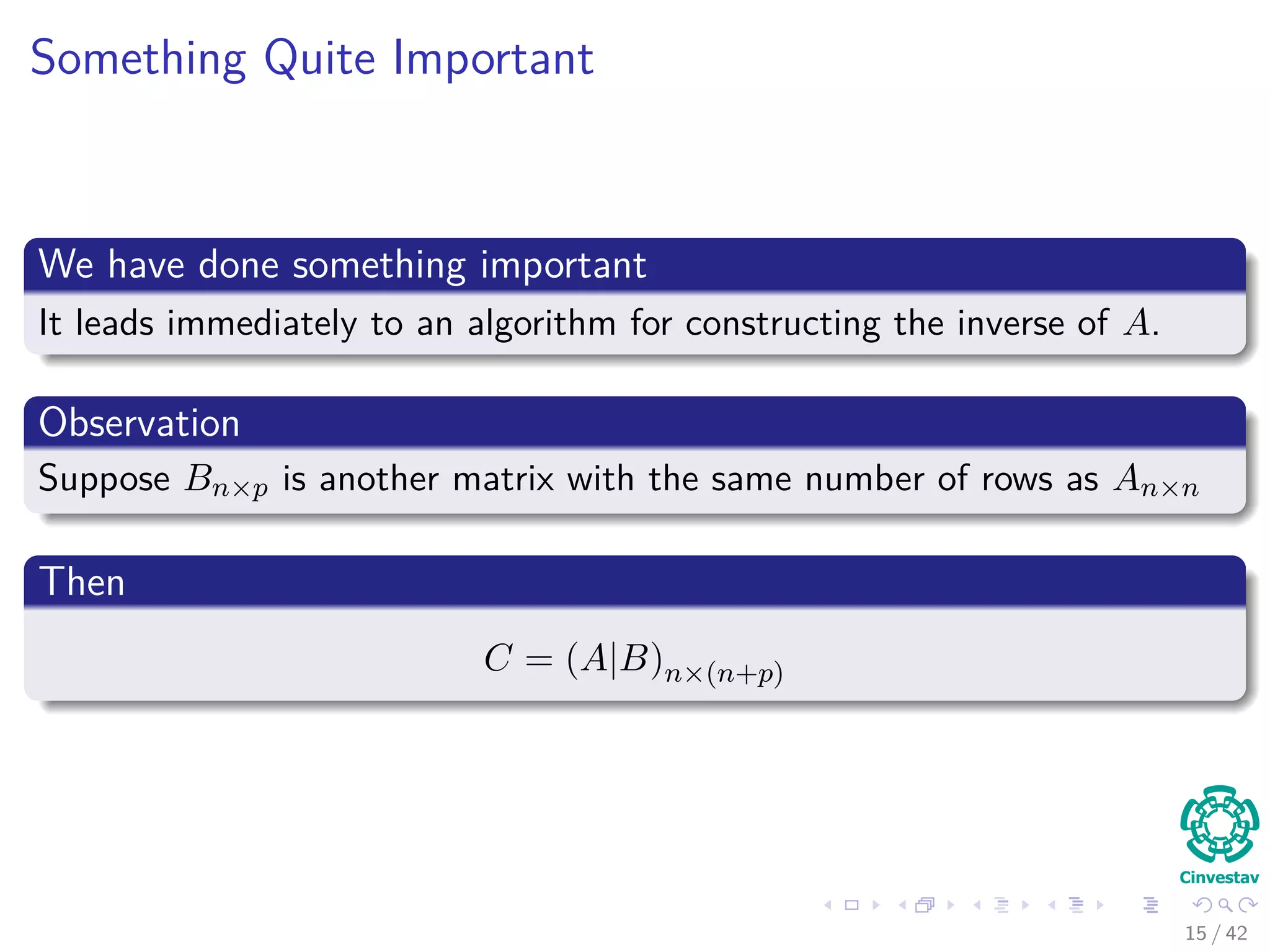
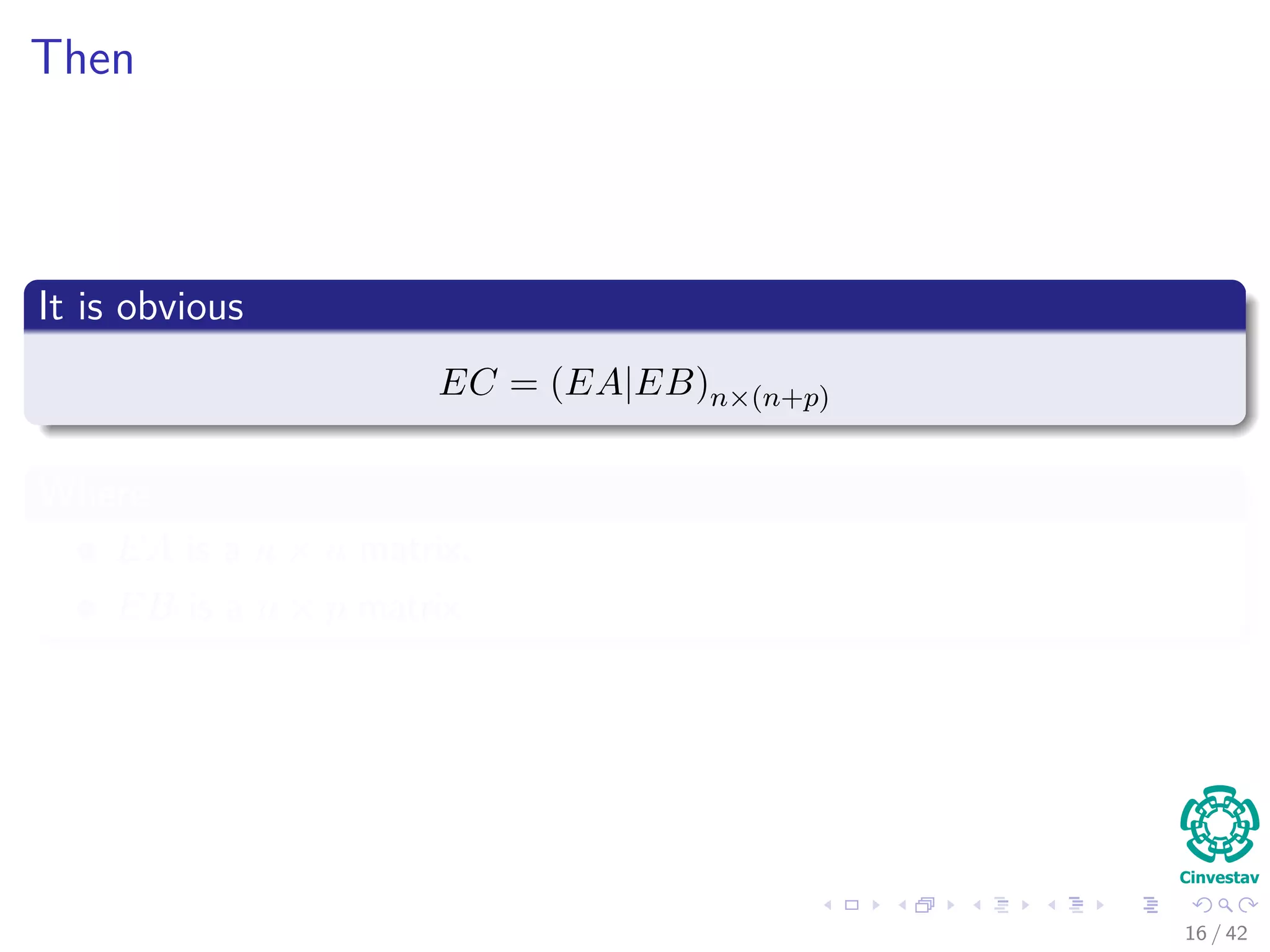
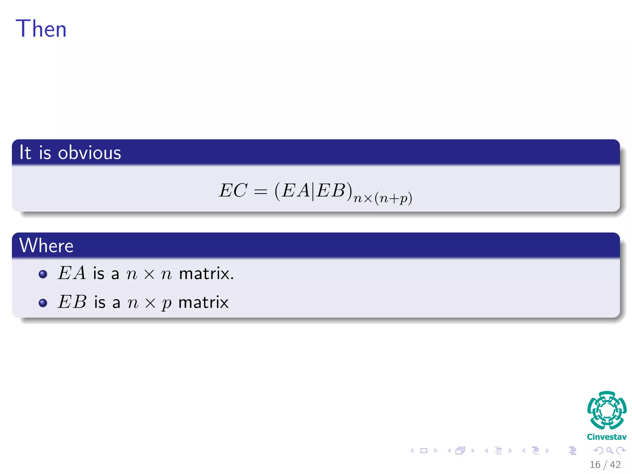
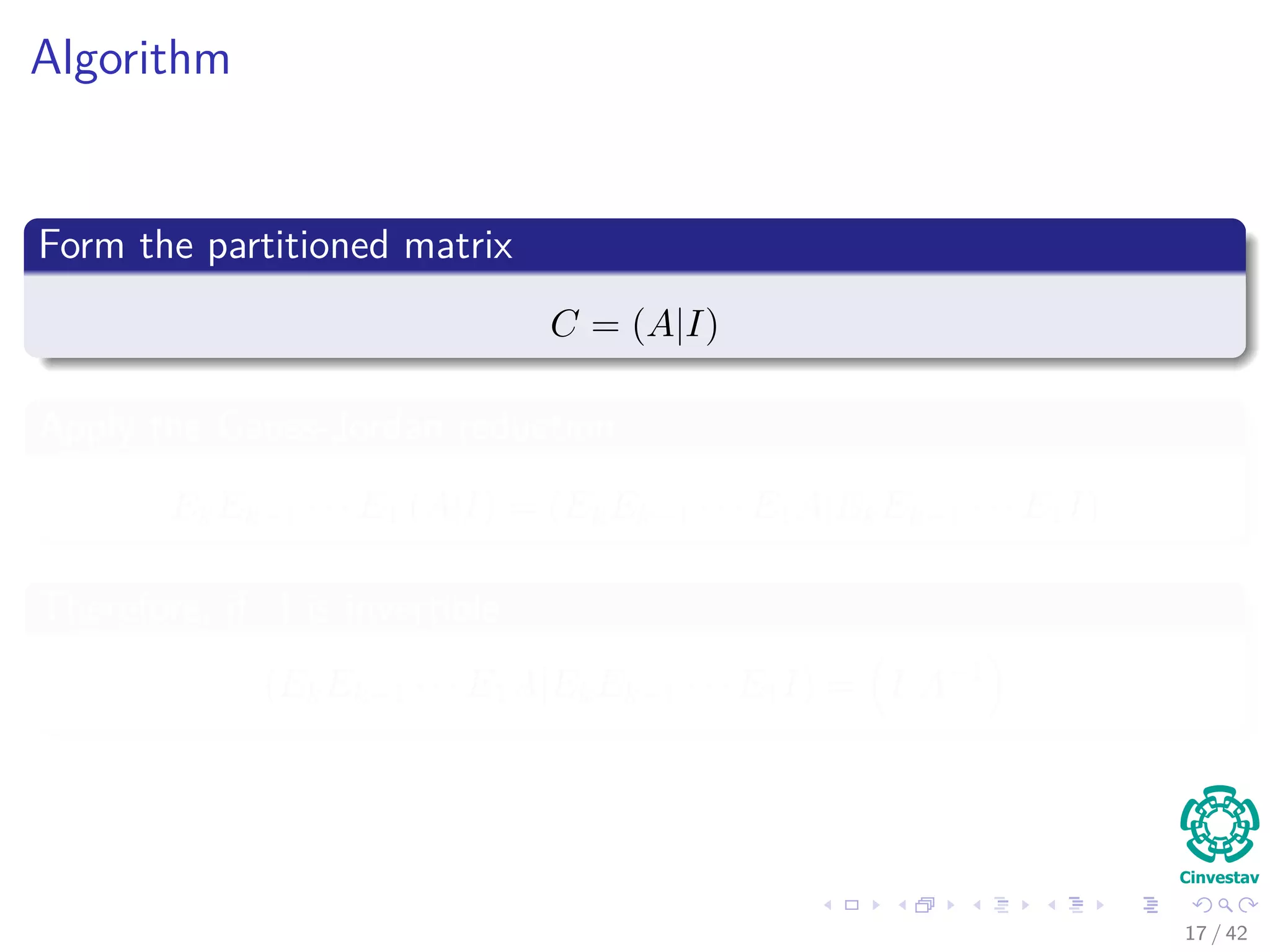
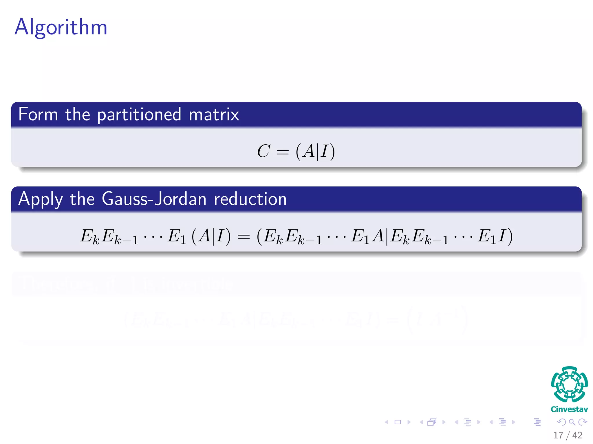
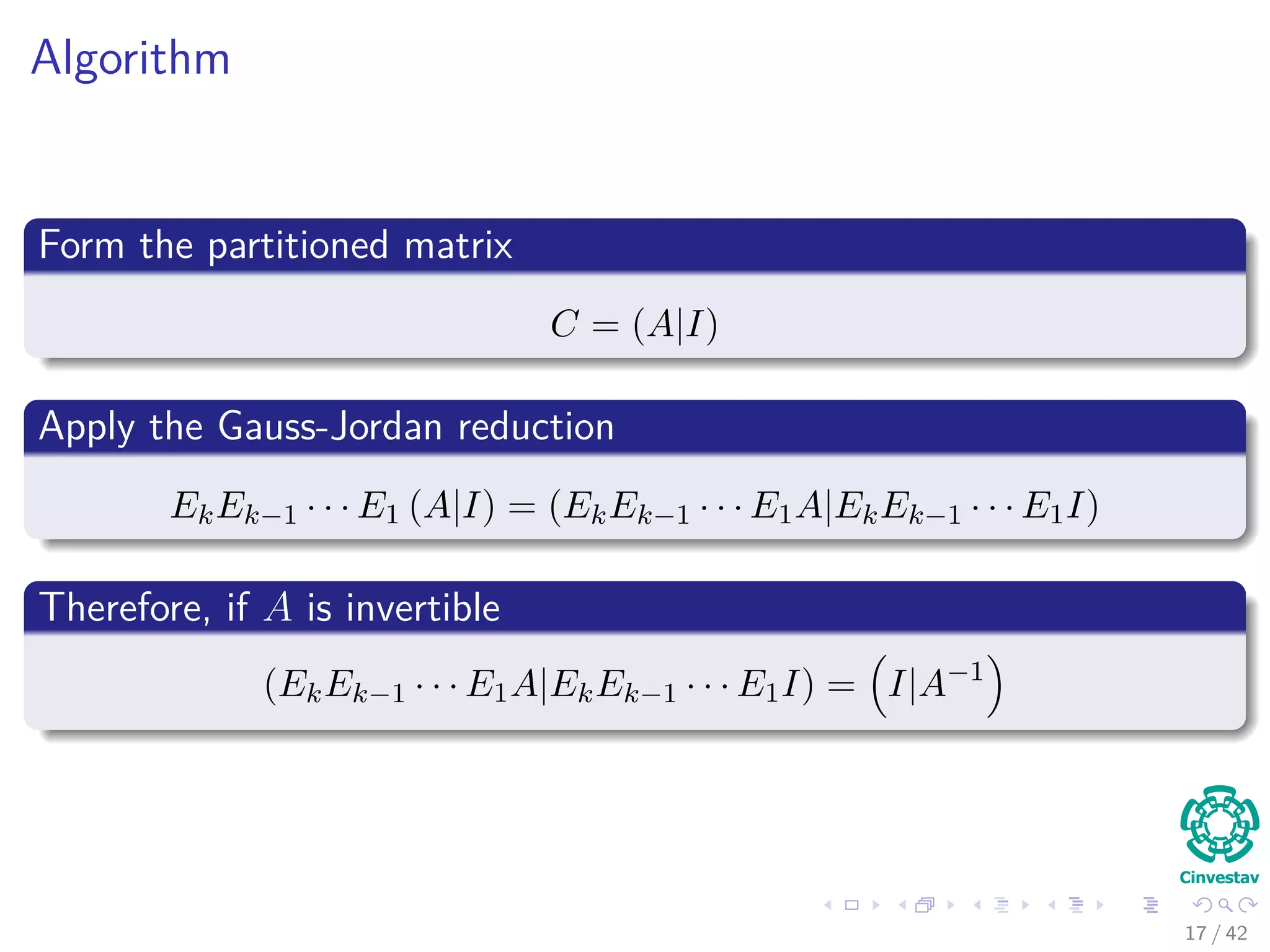
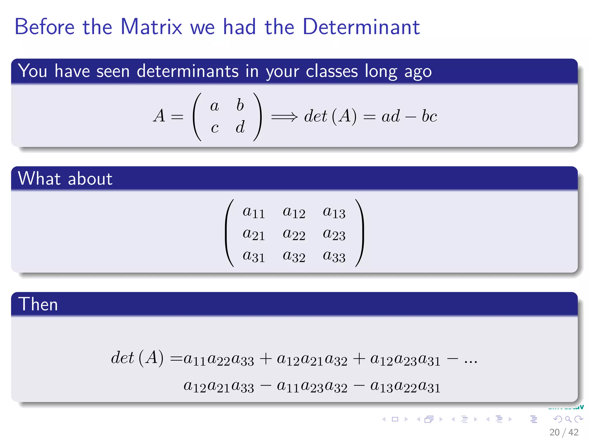
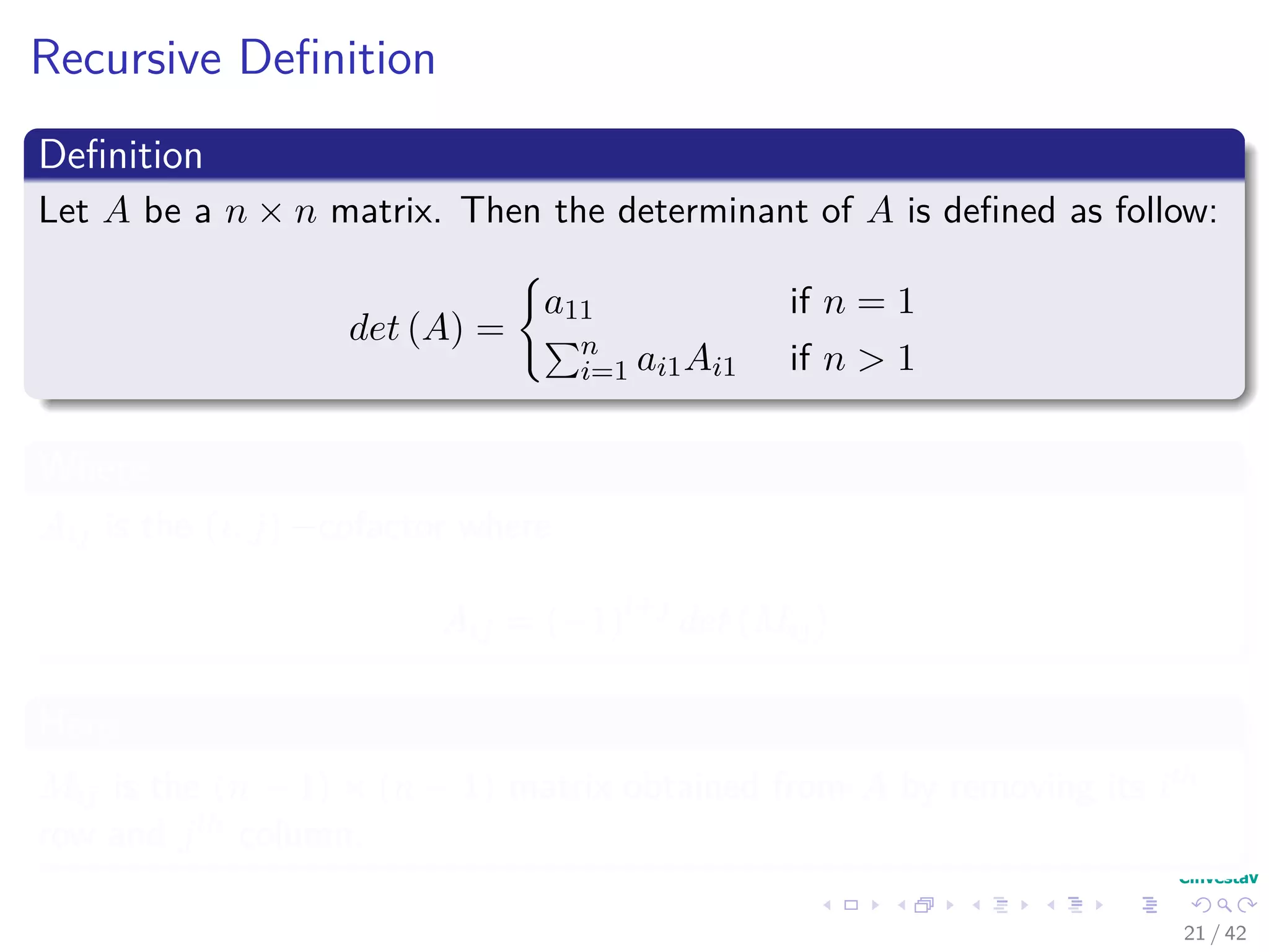
The document discusses square matrices and determinants. It begins by noting that square matrices are the only matrices that can have inverses. It then presents an algorithm for calculating the inverse of a square matrix A by forming the partitioned matrix (A|I) and applying Gauss-Jordan reduction. The document also discusses determinants, defining them recursively as the sum of products of diagonal entries with signs depending on row/column position, for matrices larger than 1x1. Complexity increases exponentially with matrix size.