Downloaded 543 times
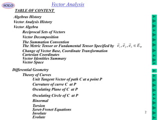
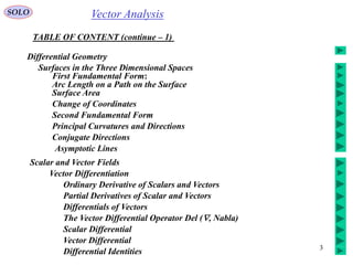
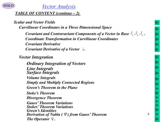
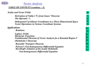
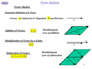
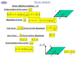
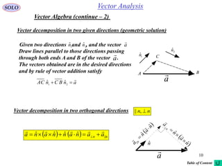
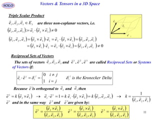
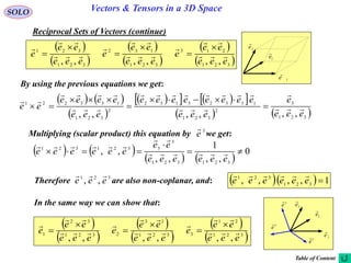
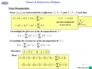
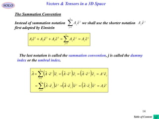
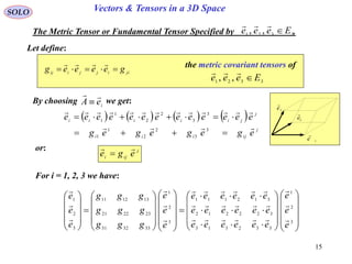
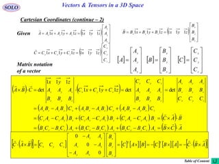
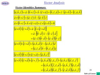
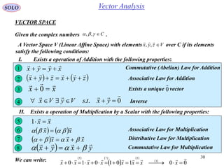
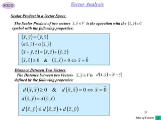


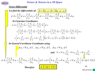
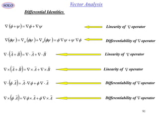
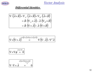
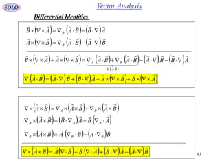
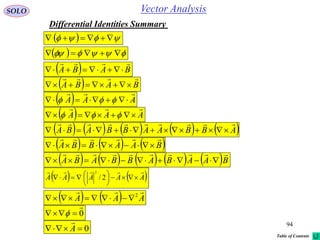
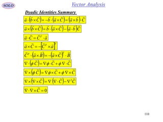
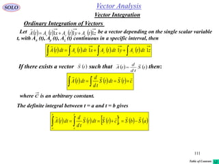
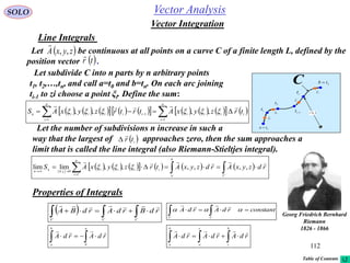
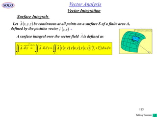
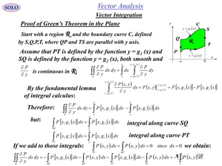
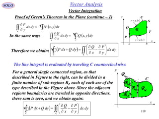
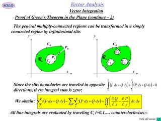
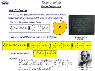
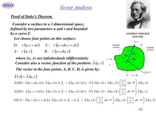
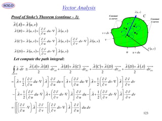
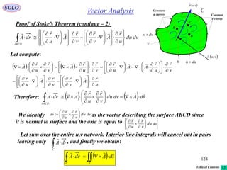
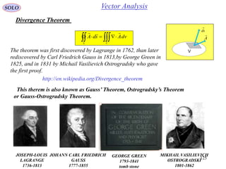
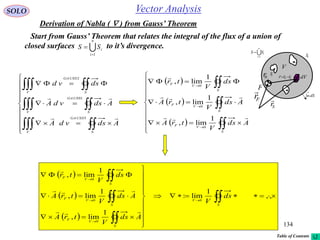
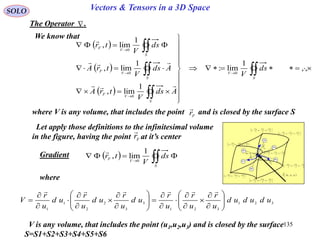
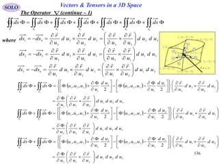
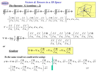
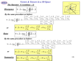
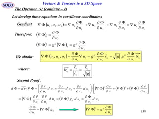
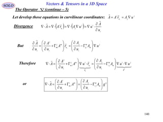
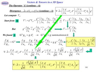
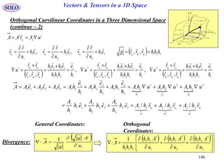
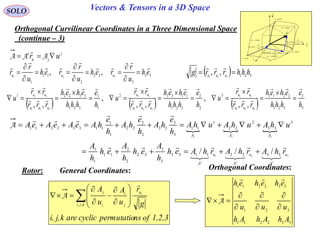
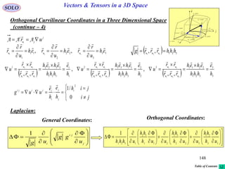
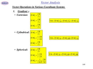
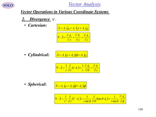
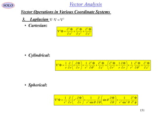
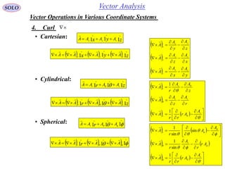
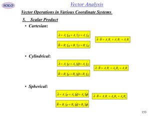
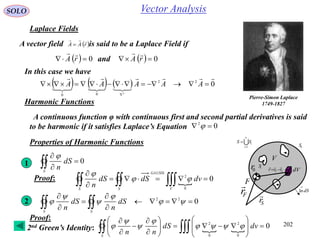
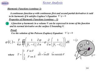
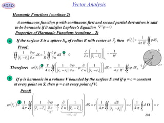

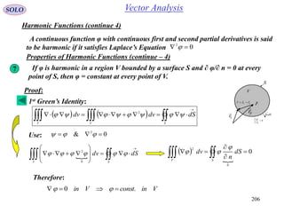
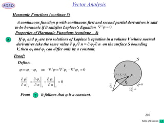
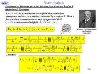
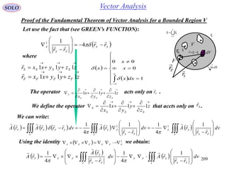
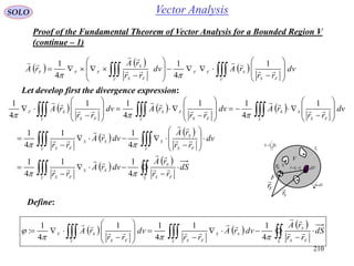
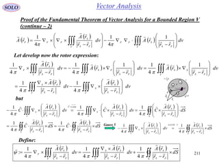
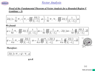
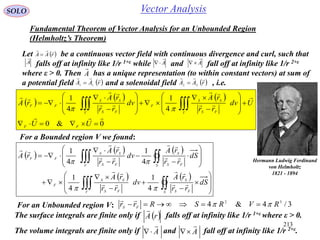
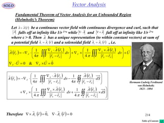
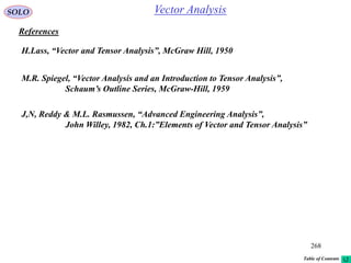


This document provides a table of contents for a textbook on vector analysis. The table of contents covers topics including: vector algebra, reciprocal sets of vectors, vector decomposition, scalar and vector fields, differential geometry, integration of vectors, and applications of vector analysis to fields such as electromagnetism and fluid mechanics. Many mathematical concepts are introduced, such as vector spaces, differential operators, vector differentiation and integration, and theorems relating concepts like divergence, curl and gradient.


![Shadechapter12.ppt [read only]](https://cdn.slidesharecdn.com/ss_thumbnails/shadechapter12-150421103821-conversion-gate02-thumbnail.jpg?width=640&height=640&fit=bounds)


![Shadechapter13.ppt [read only]](https://cdn.slidesharecdn.com/ss_thumbnails/shadechapter13-150421104054-conversion-gate02-thumbnail.jpg?width=640&height=640&fit=bounds)


