Downloaded 359 times

![8
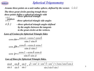
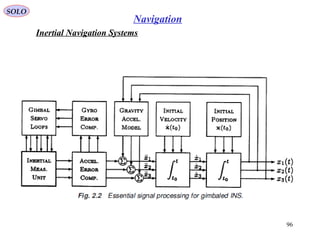
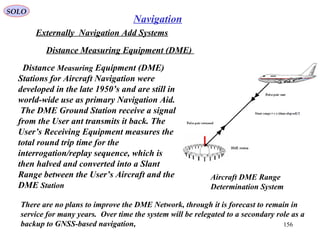
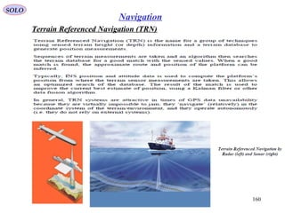
NavigationSOLO
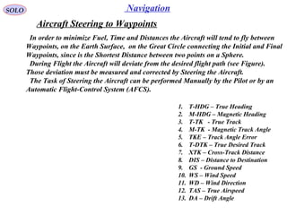
Flight on Earth Great Circles
1
2
111 ,, λφR
222 ,, λφR
The Great Circle Distance between two points 1 and
2 is ρ.
θρ ⋅= a
R – radius
- Latitudeϕ
λ - Longitude
( )
( ) ( ) ( ) ( ) ( )212121 cos90sin90sin90cos90cos
/coscos
λλφφφφ
ρθ
−⋅−⋅−+−⋅−=
=
a
From the Law of Cosines for Spherical Triangles
or
( ) ( )212121 coscoscossinsin/cos λλφφφφρ −⋅⋅+⋅=a
( ){ }212121
1
coscoscossinsincos λλφφφφρ −⋅⋅+⋅⋅= −
a
The Initial Heading Angle ψ0 can be obtained using the
Law of Cosines for Spherical Triangles as follows
( )
( )a
a
/sincos
/cossinsin
cos
1
12
0
ρφ
ρφφ
ψ
⋅
⋅−
=
( )[ ]
( )[ ]2
222
22221
coscoscossinsin1cos
coscoscossinsinsinsin
cos
λλφφφφφ
λλφφφφφφ
ψ
−⋅⋅+⋅−⋅
−⋅⋅+⋅⋅−
= −
The Heading Angle ψ from the Present Position (R, ,λ) to Destination Point (Rϕ 2,ϕ2,λ2)](https://image.slidesharecdn.com/4-navigationsystems-150812122519-lva1-app6892/85/4-navigation-systems-8-320.jpg)
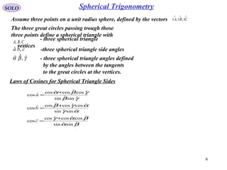
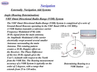
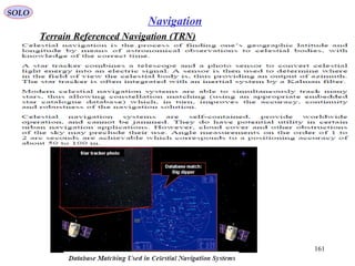
![10
NavigationSOLO
Flight on Earth Great Circles
1
2
111 ,, λφR
222 ,, λφR
If the Aircraft flies with an Heading Error Δψ we want to calculate the Down Range
Error Xd and Cross Range Error Yd, in the Spherical Triangle APB.
R – radius
- Latitudeϕ
λ - Longitude
Using the Law of Cosines for Spherical Triangle APB we have
( ) ( )aaYd /sin
90sin
/sin
sin
ρ
ψ
=
∆
( ) ( ) ( )
( ) ( ) 2/sin/sin
/cos/cos/cos
0ˆcos 21
90ˆ
RR
a
aYaX
aYaXa
P
dd
dd
P +
=
⋅
⋅−
==
= ρ
Using the Law of Sines for Spherical Triangle APB we have
( )
( )
⋅= −
aY
a
aX
d
d
/cos
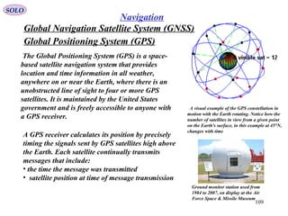
/cos
cos 1 ρ
( )[ ]ψρ ∆⋅⋅= −
sin/sinsin 1
aaYd](https://image.slidesharecdn.com/4-navigationsystems-150812122519-lva1-app6892/85/4-navigation-systems-10-320.jpg)
![19
SOLO
4. The Perifocal Coordinate System (Continue)
COORDINATES IN THE SOLAR SYSTEM
Let find a, e, ω, i, Ω from the initial position and
velocity vectors (continue).00 ,vr
The rotation matrix from the Perifocal Coordinate System Xε , Yε, Zε to the
Geocentric-Equatorial Coordinate System XG, YG, ZG is given by:
[ ] [ ] [ ]
ΩΩ−
ΩΩ
−
−=Ω=
100
0cossin
0sincos
cossin0
sincos0
001
100
0cossin
0sincos
313
ii
iiiCG
ωω
ωω
ωε
Ω−Ω
Ω+Ω−Ω−Ω−
Ω+ΩΩ−Ω
=
iii
iii
iii
cossincossinsin
sincoscoscoscossinsinsincoscoscossin
sinsincoscossinsincossincossincoscos
ωωωωω
ωωωωω](https://image.slidesharecdn.com/4-navigationsystems-150812122519-lva1-app6892/85/4-navigation-systems-19-320.jpg)
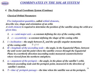
![23
SOLO
Coordinate Systems (continue – 2)
2. Earth Center Earth Fixed Coordinate –ECEF-System (E(
xE, yE in the equatorial plan with xE pointed to the intersection between the equator
to zero longitude meridian.
The Earth rotates relative to Inertial system I, with the angular velocity
sec/10.292116557.7 5
rad−
=Ω
EIIE zz
11 Ω=Ω=Ω=←ω
( )
Ω
=← 0
0
EC
IEω
Rotation Matrix from I to E
[ ]
( ) ( )
( ) ( )
ΩΩ−
ΩΩ
=Ω=
100
0cossin
0sincos
3 tt
tt
tCE
I
AIR VEHICLE IN SPHERICAL EARTH ATMOSPHERE](https://image.slidesharecdn.com/4-navigationsystems-150812122519-lva1-app6892/85/4-navigation-systems-23-320.jpg)
![25
SOLO
Coordinate Systems (continue – 4)
3.Earth Fixed Coordinate System (E0(
The origin of the system is fixed on the earth at some
given point on the Earth surface (topocentric) of
Longitude Long0 and latitude Lat0.
xE0 is pointed to the geodesic North, yE0 is pointed to the East parallel to Earth
surface, zE0 is pointed down.
[ ] [ ]
( ) ( )
( ) ( )
( ) ( )
( ) ( ) =
−
−−
−
=−−=
100
0cossin
0sincos
sin0cos
010
cos0sin
2/ 00
00
00
00
3020
0
LongLong
LongLong
LatLat
LatLat
LongLatCE
E π
( ) ( ) ( ) ( ) ( )
( ) ( )
( ) ( ) ( ) ( ) ( )
−−−
−
−−
=
00000
00
00000
sinsincoscoscos
0cossin
cossinsincossin
LatLongLatLongLat
LongLong
LatLongLatLongLat
The Angular Velocity of E relative to I is: EIIEIE zz
110 Ω=Ω== ←← ωω or
( )
( ) ( ) ( ) ( ) ( )
( ) ( )
( ) ( ) ( ) ( ) ( )
( )
( )
Ω−
Ω
=
Ω
−−−
−
−−
=
Ω
=←
0
0
00000
00
00000
00
0
sin
0
cos
0
0
sinsincoscoscos
0cossin
cossinsincossin
0
0
Lat
Lat
LatLongLatLongLat
LongLong
LatLongLatLongLat
CE
E
E
IEω
AIR VEHICLE IN SPHERICAL EARTH ATMOSPHERE
Table of Content](https://image.slidesharecdn.com/4-navigationsystems-150812122519-lva1-app6892/85/4-navigation-systems-25-320.jpg)
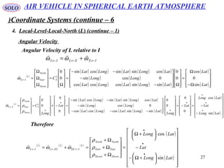
![26
SOLO
Coordinate Systems (continue – 5)
4. Local-Level-Local-North (L) or Navigation Frame
The origin of the LLLN coordinate system is located at
the projection of the center of gravity CG of the vehicle
on the Earth surface, with zDown axis pointed down,
xNorth, yEast plan parallel to the local level, with
xNorth pointed to the local North and yEast pointed to
the local East. The vehicle is located at:.
Latitude = Lat, Longitude = Long, Height = H
Rotation Matrix from E to L
[ ] [ ]
( ) ( )
( ) ( )
( ) ( )
( ) ( ) =
−
−−
−
=−−=
100
0cossin
0sincos
sin0cos
010
cos0sin
2/ 32 LongLong
LongLong
LatLat
LatLat
LongLatCL
E π
( ) ( ) ( ) ( ) ( )
( ) ( )
( ) ( ) ( ) ( ) ( )
−−−
−
−−
=
LatLongLatLongLat
LongLong
LatLongLatLongLat
sinsincoscoscos
0cossin
cossinsincossin
AIR VEHICLE IN SPHERICAL EARTH ATMOSPHERE](https://image.slidesharecdn.com/4-navigationsystems-150812122519-lva1-app6892/85/4-navigation-systems-26-320.jpg)
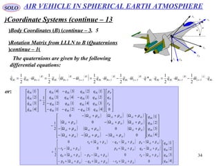
![31
SOLO
Coordinate Systems (continue – 10)
5.Body Coordinates (B(
The origin of the Body coordinate system
is located at the instantaneous center of
gravity CG of the vehicle, with xB pointed
to the front of the Air Vehicle, yB pointed
toward the right wing and zB completing
the right-handed Cartesian reference frame.
Rotation Matrix from LLLN to B (Euler Angles(:
[ ] [ ] [ ]
−+
+−
−
==
θφψφψθφψφψθφ
θφψφψθφψφψθφ
θψθψθ
ψθφ
cccssscsscsc
csccssssccss
ssccc
CB
L 321
ψ - azimuth angle
θ - pitch angle
φ - roll angle
AIR VEHICLE IN SPHERICAL EARTH ATMOSPHERE](https://image.slidesharecdn.com/4-navigationsystems-150812122519-lva1-app6892/85/4-navigation-systems-31-320.jpg)
![32
SOLO
Coordinate Systems (continue – 11)
5.Body Coordinates (B( (continue – 1( ψ
θ
φ Bx
Lx
Bz
Ly
Lz
By
Angular Velocity from L to B (Euler Angles(:
( )
[ ] [ ] [ ]
+
+
=
=←
ψ
θφθφ
φ
ω
0
0
0
0
0
0 211
R
Q
P
B
LB
−
−
+
−
+
=
ψθθ
θθ
φφ
φφθ
φφ
φφ
φ
0
0
cos0sin
010
sin0cos
cossin0
sincos0
001
0
0
cossin0
sincos0
001
0
0
[ ]
=
−
−
=
ψ
θ
φ
ψ
θ
φ
θφφ
θφφ
θ
G
coscossin0
cossincos0
sin01
AIR VEHICLE IN SPHERICAL EARTH ATMOSPHERE](https://image.slidesharecdn.com/4-navigationsystems-150812122519-lva1-app6892/85/4-navigation-systems-32-320.jpg)
![33
SOLO
Coordinate Systems (continue – 12)
5.Body Coordinates (B( (continue – 2( ψ
θ
φ Bx
Lx
Bz
Ly
Lz
By
Rotation Matrix from LLLN to B (Quaternions(:
( ) [ ][ ] ( ) [ ][ ] { } { }
( ) ( ) ( ) ( )
( ) ( ) ( ) ( )
( ) ( ) ( ) ( )
( ) ( ) ( )
( ) ( ) ( )
( ) ( ) ( )
( ) ( ) ( )
−−−
−
−
−
−−
−−
−−
=
+×−×−=
321
412
143
234
3412
2143
1234
44 3333
BIBLBL
BLBLBL
BLBLBL
BLBLBL
BLBLBLBL
BLBLBIBL
BLBLBLBL
T
BLBLBLXBLBLXBL
B
L
qqq
qqq
qqq
qqq
qqqq
qqqq
qqqq
qqqIqqIqC
where: ( )
( )
( )
( )
( )
( )
( )
( )
{ }
( )
{ }
( )
( )
( )
=
=
=
=
3
2
1
:&
4
4
3
2
1
4
3
2
1
BL
BL
BL
BL
BL
BL
BL
BL
BL
BL
BL
BL
BL
BL
BL
BL
q
q
q
q
q
q
qor
q
q
q
q
q
q
q
q
q
( )
−
=
2
sin
2
sin
2
sin
2
cos
2
cos
2
cos4
ϕθψϕθψ
BLq
( )
+
=
2
cos
2
sin
2
sin
2
sin
2
cos
2
cos1
ϕθψϕθψ
BLq
( )
−
=
2
sin
2
cos
2
sin
2
cos
2
sin
2
cos2
ϕθψϕθψ
BLq
( )
+
=
2
sin
2
sin
2
cos
2
cos
2
cos
2
sin3
ϕθψϕθψ
BLq
AIR VEHICLE IN SPHERICAL EARTH ATMOSPHERE](https://image.slidesharecdn.com/4-navigationsystems-150812122519-lva1-app6892/85/4-navigation-systems-33-320.jpg)
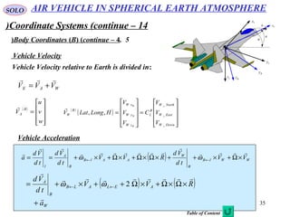
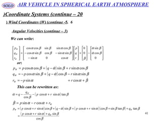
![36
SOLO
Coordinate Systems (continue – 15)
6.Wind Coordinates (W(
The origin of the Wind coordinate system
is located at the instantaneous center of
gravity CG of the vehicle, with xW pointed
in the direction of the vehicle velocity vector
relative to air .AV
[ ] [ ]
−
−−=
−
−=−=
αα
βαββα
βαββα
αα
αα
ββ
ββ
αβ
cos0sin
sinsincossincos
cossinsincoscos
cos0sin
010
sin0cos
100
0cossin
0sincos
23
W
BC
The Wind coordinate frame is defined by the following two angles:
α - angle of attack
β - sideslip angle
AIR VEHICLE IN SPHERICAL EARTH ATMOSPHERE](https://image.slidesharecdn.com/4-navigationsystems-150812122519-lva1-app6892/85/4-navigation-systems-36-320.jpg)
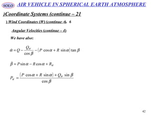
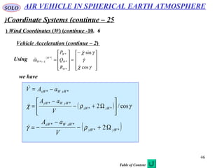
![37
SOLO
Coordinate Systems (continue – 16)
6.Wind Coordinates (W( (continue -1(
Rotation Matrix from L (LLLN) to W is:
χ - azimuth angle of the trajectory
γ - pitch angle of the trajectory
Rotation Matrix
[ ] [ ] [ ] [ ] [ ] 32123 ψθφαβ −== B
L
W
B
W
L CCC
The Rotation Matrix from L (LLLN) to W can also be defined by the following
Consecutive rotations:
σ - bank angle of the
trajectory
[ ] [ ] [ ] [ ]
−+
+−
−
===
γσχσχγσχσχγσ
γσχσχγσχσχγσ
γχγχγ
χγσσ
cccssscsscsc
csccssssccss
ssccc
CC W
L
W
L 321
*
1
We defined also the intermediate wind frame W* by:
[ ] [ ]
−
−
==
γχγχγ
χχ
γχγχγ
χγ
csscs
cs
ssccc
CW
L 032
*
AIR VEHICLE IN SPHERICAL EARTH ATMOSPHERE](https://image.slidesharecdn.com/4-navigationsystems-150812122519-lva1-app6892/85/4-navigation-systems-37-320.jpg)
![38
SOLO
Coordinate Systems (continue – 17)
6.Wind Coordinates (W( (continue -2(
Angular Velocity of W* relative to LLLN is:
Angular Velocities
( )
[ ]
−
=
−
+
=
+
=
=←
γχ
γ
γχ
χγγ
γγ
γ
χ
γγω
cos
sin
0
0
cos0sin
010
sin0cos
0
0
0
0
0
0
2
*
*
*
*
*
W
W
W
W
LW
R
Q
P
Angular Velocity of W relative to LLLN is:
( )
[ ] [ ]
−
−
=
−
−
+
=
+
+
=
=←
χ
γ
σ
γσσ
γσσ
γ
γχ
γ
γχ
σσ
σσ
σ
χ
γγσ
σ
ω
coscossin0
cossincos0
sin01
cos
sin
cossin0
sincos0
001
0
00
0
0
0
0
0 21
W
W
W
W
LW
R
Q
P
AIR VEHICLE IN SPHERICAL EARTH ATMOSPHERE](https://image.slidesharecdn.com/4-navigationsystems-150812122519-lva1-app6892/85/4-navigation-systems-38-320.jpg)
![39
SOLO
Coordinate Systems (continue – 18)
6.Wind Coordinates (W( (continue -3(
We have also:
Angular Velocities (continue – 1(
( ) ( )
( )
( )
Ω
Ω
Ω
=
Ω−
Ω
==
Ω
Ω
Ω
= ←←
Down
East
North
W
L
W
L
L
IE
W
L
zW
yW
xW
W
IE C
Lat
Lat
CC ***
*
*
*
*
sin
0
cos
ωω
( ) ( )
( )
( )
=
−
−==
=
•
•
•
←←
Down
East
North
W
L
W
L
L
EL
W
L
zW
yW
xW
W
EL C
LatLong
Lat
LatLong
CC
ρ
ρ
ρ
ω
ρ
ρ
ρ
ω ***
*
*
*
*
sin
cos
( ) ( )
( )
( )
[ ] ( )*
1
sin
0
cos
W
IE
W
L
L
IE
W
L
zW
yW
xW
W
IE
Lat
Lat
CC ←←← =
Ω−
Ω
==
Ω
Ω
Ω
= ωσωω
( ) ( )
( )
( )
[ ] ( )*
1
sin
cos
W
IL
W
L
L
IL
W
L
W
IL
LatLong
Lat
LatLong
CC ←
•
•
•
←← =
+Ω−
−
+Ω
== ωσωω
AIR VEHICLE IN SPHERICAL EARTH ATMOSPHERE](https://image.slidesharecdn.com/4-navigationsystems-150812122519-lva1-app6892/85/4-navigation-systems-39-320.jpg)
![40
SOLO
Coordinate Systems (continue – 19)
6.Wind Coordinates (W( (continue -4(
The Angular Velocity from I to W is:
Angular Velocities (continue – 2(
( ) ( ) ( ) ( )
Ω+
Ω+
Ω+
+
=+
=+=
= ←←←←
DownDown
EastEast
NorthNorth
W
L
W
W
W
L
IL
W
L
W
W
W
W
IL
W
LW
W
W
W
W
IW C
R
Q
P
C
R
Q
P
r
q
p
ρ
ρ
ρ
ωωωω
Using the angle of attack α and the sideslip angle β , we can write:
BWBW yz
11 αβω −=←
or:
( ) ( ) ( )
[ ]
−
=
−
=−= ←←←
0
0
0
0
3 αβ
β
ωωω
r
q
p
C
r
q
p
W
B
W
W
W
W
IB
W
IW
W
BW
but also:
( ) ( ) ( )
[ ]
−
=
−
=−= ←←←
0
0
0
0
3 αβ
β
ωωω
R
Q
P
C
R
Q
P
W
B
W
W
W
W
LB
W
LW
W
BW
AIR VEHICLE IN SPHERICAL EARTH ATMOSPHERE](https://image.slidesharecdn.com/4-navigationsystems-150812122519-lva1-app6892/85/4-navigation-systems-40-320.jpg)
![43
SOLO
Coordinate Systems (continue – 22)
6.Wind Coordinates (W( (continue -7(
The vehicle velocity was decomposed in:
Vehicle Velocity
WAE VVV
+=
( )
=
0
0
V
V
W
A
- vehicle velocity relative to atmosphere
( )
( )
=
=
DownW
EastW
NorthW
W
L
zW
yW
xW
W
W
V
V
V
C
V
V
V
HLongLatV
W
W
W
_
_
_
,,
- wind velocity at velocity position
also
( )
[ ] ( )
[ ]
=
−=−=
0
0
0
011
*
VV
VV
W
A
W
A σσ
( )
( )
=
=
DownW
EastW
NorthW
W
L
zW
yW
xW
W
W
V
V
V
C
V
V
V
HLongLatV
W
W
W
_
_
_
*
*
*
*
*
,,
AIR VEHICLE IN SPHERICAL EARTH ATMOSPHERE](https://image.slidesharecdn.com/4-navigationsystems-150812122519-lva1-app6892/85/4-navigation-systems-43-320.jpg)
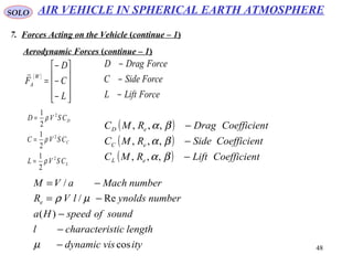
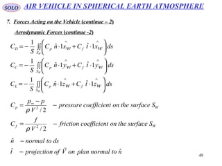
![47
SOLO
Aerodynamic Forces
( )[ ]∫∫ +−= ∞
WS
A dstfnppF
11
ntonormalplanonVofprojectiont
dstonormaln
ˆˆ
ˆ
−
−
( )
airflowingthebyweatedsurfaceVehicleS
SsurfacetheonmNstressforcefrictionf
Ssurfacetheondifferencepressurepp
W
W
W
−
−
−−∞
)/( 2
AIR VEHICLE IN SPHERICAL EARTH ATMOSPHERE
7. Forces Acting on the Vehicle](https://image.slidesharecdn.com/4-navigationsystems-150812122519-lva1-app6892/85/4-navigation-systems-47-320.jpg)
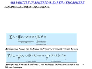
![51
SOLO
( ) ( ) ( )∫∫ −++= ∞
<> iopenS
outflowoutopenflowinflowinopenflow dsnppmVmVT
1:
0
/
0
/ THRUST FORCES
( ) ( ) ( ) ( )[ ]∫∫ −×−+×−−×−= ∞
<> iopenS
OoutflowoutopenflowCoutopeninflowinopenflowCiopenCT dsnppRRmVRRmVRRM
1:
0
/
0
/,
THRUST MOMENTS
RELATIVE TO C
( ) ( )∫∫ −+ ∞
> inopenS
inflowinopenflow dsnppmV
1
00
/
( ) ( )∫∫ −+ ∞
< outopenS
outflowoutopenflow dsnppmV
1
0
/
T
outopenR
iopenR
CR
C
AIR VEHICLE IN SPHERICAL EARTH ATMOSPHERE
Table of Content](https://image.slidesharecdn.com/4-navigationsystems-150812122519-lva1-app6892/85/4-navigation-systems-51-320.jpg)
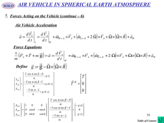
![52
SOLO
7. Forces Acting on the Vehicle (continue – 3)
Thrust
( ) ( )
−
−−==
B
B
B
z
y
x
BW
B
W
T
T
T
TCT
αα
βαββα
βαββα
cos0sin
sinsincossincos
cossinsincoscos
**
( )
[ ] ( )
−
==
=
*
*
*
cossin0
sincos0
001
*
1
W
W
W
W
W
W
z
y
x
W
z
y
x
W
T
T
T
T
T
T
T
T
σσ
σσσ
AIR VEHICLE IN SPHERICAL EARTH ATMOSPHERE
F-35Thrust Vector Control](https://image.slidesharecdn.com/4-navigationsystems-150812122519-lva1-app6892/85/4-navigation-systems-52-320.jpg)
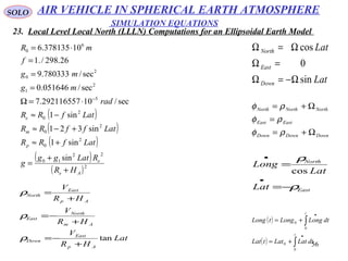
![53
SOLO
7. Forces Acting on the Vehicle (continue – 4)
Gravitation Acceleration
( ) ( )
−
−
−
==
zg
yg
xg
gg
100
0
0
0
010
0
0
0
001
χχ
χχ
γγ
γγ
σσ
σσ cs
sc
cs
sc
cs
scC EW
E
W
( )
gg
−
=
γσ
γσ
γ
cc
cs
s
W
2sec/174.322sec/81.9
0
2
0
0
0
gg ftmg
HR
R
==
+
=
AIR VEHICLE IN SPHERICAL EARTH ATMOSPHERE
The derivation of Gravitation Acceleration assumes an Ellipsoidal Symmetrical Earth.
The Gravitational Potential U (R, ( is given byϕ
( ) ( )
( )
( )φ
φ
µ
φ
,
sin1, 2
RUg
P
R
a
J
R
RU
E
E
n n
n
n
∇=
−⋅−= ∑
∞
=
μ – The Earth Gravitational Constant
a – Mean Equatorial Radius of the Earth
R=[xE
2
+yE
2
+zE
2
]]/2
is the magnitude of
the Geocentric Position Vector
– Geocentric Latitude (sin =zϕ ϕ E/R(
Jn – Coefficients of Zonal Harmonics of the
Earth Potential Function
P (sin ( – Associated Legendre Polynomialsϕ](https://image.slidesharecdn.com/4-navigationsystems-150812122519-lva1-app6892/85/4-navigation-systems-53-320.jpg)


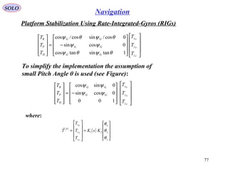
![SOLO
75
Navigation
Platform Stabilization Using Rate-Integrated-Gyros (RIGs(
The Platform is angular isolated from the Aircraft
via, at least, three Gimbals. Those Gimbals are,
from Aircraft to Platform:
- Azimuth (Heading( – Angle ψG
- Pitch – Angle θ
- Roll – Angle ϕ
The Rotation Matrix from Aircraft to Platform is:
[ ] [ ] [ ]
−
−
−
==
100
0cossin
0sincos
cos0sin
010
sin0cos
cossin0
sincos0
001
321 GG
GG
G
P
AC ψψ
ψψ
θθ
θθ
φφ
φφψθφ
We want to apply Moments on the Platform, related to the Pjckoff
Outputs
of the Three RIGs mounted on the Platform
( )
( )
=
=
z
y
x
z
y
x
P
KsK
T
T
T
T
P
P
P
θ
θ
θ
21
The 3 Torque Motors Roll (TR(, Pitch (TP( and Heading (TH(
are located on Gimbal Axes .PA zyx 1,1,1 '
](https://image.slidesharecdn.com/4-navigationsystems-150812122519-lva1-app6892/85/4-navigation-systems-75-320.jpg)
![SOLO
76
Navigation
Platform Stabilization Using Rate-Integrated-Gyros (RIGs(
We want to find the relation between and
TR, TP, TH.
PPP zyx TTT ,,
The 3 Torque Motors Roll (TR(, Pitch (TP( and Heading (TH(
are located on Gimbal Axes .PA zyx 1,1,1 '
PAPPPPPP zHyPxRzzyyxx TTTTTTT 111111 '
++=++=
( )
[ ] [ ] [ ]
( )
[ ] [ ]
( )
[ ]
( )
P
Pzy
A
Ax
P
P
P
GHGPGR
z
y
x
P
TTT
T
T
T
T
1
3
1
23
1
123
1
0
0
0
1
0
0
0
1
,
'
−+
−−+
−−−=
= ψθψφθψ
−
−
=
H
P
R
GG
GG
z
y
x
T
T
T
T
T
T
P
P
P
10sin
0coscossin
0sincoscos
θ
ψθψ
ψθψ
−=
P
P
P
z
y
x
GG
GG
GG
H
P
R
T
T
T
T
T
T
1tansintancos
0cossin
0cos/sincos/cos
θψθψ
ψψ
θψθψ](https://image.slidesharecdn.com/4-navigationsystems-150812122519-lva1-app6892/85/4-navigation-systems-76-320.jpg)
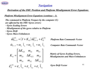
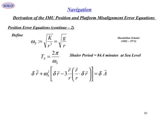
![SOLO
79
Navigation
Derivation of the IMU Position and Platform Misalignment Error Equations
Platform Misalignment Error Equations
Define:
(C(Computer Coordinate System
(the computed Platform coordinates(
(P( Platform Coordinate System
(real Platform coordinates(
The rotation from (C( to (P( is defined by
the three small angles ψx, ψy, ψz as
[ ] [ ] [ ]
−
−
−
==
100
0cossin
0sincos
cos0sin
010
sin0cos
cossin0
sincos0
001
321 zz
zz
yy
yy
xx
xxzyx
P
CC ψψ
ψψ
ψψ
ψψ
ψψ
ψψψψψ
−
−
−
−
=
−
−
−
≈
−
−
−
≈
0
0
0
100
010
001
1
1
1
100
01
01
10
010
01
10
10
001
xy
xz
yz
xy
xz
yz
z
z
y
y
x
x
ψψ
ψψ
ψψ
ψψ
ψψ
ψψ
ψ
ψ
ψ
ψ
ψ
ψ
[ ] [ ] [ ]
−
−
−
=×
=×−≈
0
0
0
:&:
xy
xz
yz
z
y
x
P
C IC
ψψ
ψψ
ψψ
ψ
ψ
ψ
ψ
ψψ
](https://image.slidesharecdn.com/4-navigationsystems-150812122519-lva1-app6892/85/4-navigation-systems-79-320.jpg)
![SOLO
80
Navigation
Derivation of the IMU Position and Platform Misalignment Error Equations
Platform Misalignment Error Equations (continue – 1(
Let find the angular rotation vector from C to P
( )
[ ] [ ] [ ] =
+
+
=←
z
zyy
x
x
P
CP
ψ
ψψψ
ψ
ψω
0
0
0
0
0
0 321
ψ
ψ
ψ
ψ
ψ
ψψψ
ψψψ
ψψψ
ψψ
ψψ
ψ
ψ
ψψ
=
≈
+
−
=
−
−
−
+
−
+
≈
z
y
x
z
zxy
zyx
zxy
xz
yz
y
y
yx
0
0
1
1
1
0
0
10
010
01
0
0](https://image.slidesharecdn.com/4-navigationsystems-150812122519-lva1-app6892/85/4-navigation-systems-80-320.jpg)
![SOLO
82
Navigation
Derivation of the IMU Position and Platform Misalignment Error Equations
Platform Misalignment Error Equations (continue – 2(
Let find the angular velocity vector of the Platform (P(
relative to the Computer (C(:
ICIPCP ←←← −= ωωω
( ) ( ) ( ) ( ) ( )C
IC
P
C
P
IP
P
IC
P
IP
P
CP C ←←←←← −=−= ωωωωω
( ) ( ) ( )
[ ]{ } ( )
[ ] ( ) ( ) ( )P
G
C
ICG
C
IC
C
IC
P
G
C
ICG KIKI εωωψωψεωψ
++×=×−−++= ←←←←
Using we obtain:[ ] ( ) ( )
[ ] ψωωψ
×−=× ←←
C
IC
C
IC
( )
[ ] ( ) ( )P
G
C
ICG
C
IC K εωψωψ
++×−= ←←
or
+
∆
∆
∆
+
−
−
−
−=
z
y
x
z
y
x
G
G
G
z
y
x
xy
xz
yz
z
y
x
C
C
C
CC
CC
CC
Kmm
mKm
mmK
ε
ε
ε
ω
ω
ω
ψ
ψ
ψ
ωω
ωω
ωω
ψ
ψ
ψ
33231
23221
13121
0
0
0
](https://image.slidesharecdn.com/4-navigationsystems-150812122519-lva1-app6892/85/4-navigation-systems-82-320.jpg)
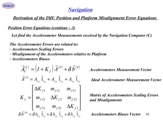
![SOLO
84
Navigation
Derivation of the IMU Position and Platform Misalignment Error Equations
Position Error Equations (continue – 1(
( ) ( )rgrrgAr
−++= δδδ
( ) ( )
( ) ( )[ ]
r
r
K
r
rrrr
K
rgrrg
32/3
+
+⋅+
−=−+
δδ
δ
( )
( ) r
r
K
r
rr
rr
r
K
r
r
K
r
rrr
K
32332/32
31
2
+
⋅
−+−≈+
⋅+
−≈
δ
δ
δ
r
r
K
r
r
r
r
r
r
K
r
r
K
r
r
K
3333
+
⋅+−−≈ δδ
therefore
Ar
r
r
r
r
r
r
K
r
δδδδ =
⋅−+ 33](https://image.slidesharecdn.com/4-navigationsystems-150812122519-lva1-app6892/85/4-navigation-systems-84-320.jpg)
 ( )PPP
f
PC
P
C
C
C
AIbAKIACAA
×+−++=−= ψδδ
We used the relation ( ) [ ]( ) [ ]( )×+≈×−==
−−
ψψ
IICC P
C
C
P
11
Finally we obtain
( )
[ ] ( ) ( ) ( )PP
f
PC
bAKAA
δψδ ++×−=
[ ] ( ) ( ) ( )PP
f
P
S bAKAr
r
r
r
r
rr
δψδδωδ ++×−=
⋅−+ 32
The Position Error Equation is](https://image.slidesharecdn.com/4-navigationsystems-150812122519-lva1-app6892/85/4-navigation-systems-87-320.jpg)
![SOLO
88
Navigation
Derivation of the IMU Position and Platform Misalignment Error Equations
Position Error Equations (continue – 5(
Let compute ( )C
r
δ
( ) ( ) ( )
[ ] ( )CC
IC
CC
rrr
δωδδ ×+= ←
Therefore
( )
( )
( )
( ) ( )
CCCCCC
CCC
C
IC
C
CCC
CCC
CCCCCC
CCC
zzyyxxIC
C
ICzyxICzyx
zyx
C
zyxzyx
C
zyx
C
rzyxzyx
zyxr
zyxzyxr
zyxr
111
111111
111:
111111
111
11
ωωωω
δωδδδωδδδ
δδδδ
δδδδδδδ
δδδδ
αα
ω
++=
×=++×=++
++=
+++++=
++=
←
←←
×= ←
In the same way
( ) ( ) ( )
[ ] ( ) ( ) ( )
[ ] ( ) ( )
( )
[ ] ( ) ( )
[ ] ( )
( )CC
IC
CC
IC
CC
IC
C
IC
C
IC
CC
IC
CC
rr
rrrr
δωδω
δωωωδωδδ
×+×+
×
×++×+=
←←
←←←←
0](https://image.slidesharecdn.com/4-navigationsystems-150812122519-lva1-app6892/85/4-navigation-systems-88-320.jpg)
![SOLO
89
Navigation
Derivation of the IMU Position and Platform Misalignment Error Equations
Position Error Equations (continue – 6(
( ) ( ) ( )
[ ] ( )CC
IC
CC
rrr
δωδδ ×+= ←
Therefore
( ) ( ) ( )
[ ] ( ) ( )
[ ] ( )
[ ] ( )
[ ]( ) ( )CC
IC
C
IC
C
IC
CC
IC
CC
rrrr
δωωωδωδδ ××+×+×+= ←←←←2
( ) ( )
[ ] ( ) ( )
[ ] ( )
[ ] ( )
[ ]( ) ( ) ( )
( ) ( )
( )
[ ] ( ) ( ) ( )PP
f
P
C
CC
C
S
CC
IC
C
IC
C
IC
CC
IC
C
bAKA
r
r
r
r
r
rrrr
δψ
δδωδωωωδωδ
++×−=
⋅−+××+×+×+ ←←←← 32 2
Together with the Platform Misalignment Error Equations
( )
[ ] ( ) ( )P
G
C
ICG
C
IC K εωψωψ
++×−= ←←](https://image.slidesharecdn.com/4-navigationsystems-150812122519-lva1-app6892/85/4-navigation-systems-89-320.jpg)
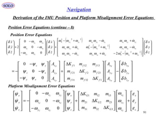
![SOLO
90
Navigation
Derivation of the IMU Position and Platform Misalignment Error Equations
Position Error Equations (continue – 7(
CCCCCC zzyyxxIC 111
ωωωω ++=←
( )
[ ]
−
−
−
=×←
0
0
0
CC
CC
CC
xy
xz
yz
C
IC
ωω
ωω
ωω
ω
( )
[ ]
−
−
−
=×←
0
0
0
CC
CC
CC
xy
xz
yz
C
IC
ωω
ωω
ωω
ω
( )
[ ] ( )
[ ]
( )
( )
( )
+−
+−
+−
=
−
−
−
−
−
−
=×× ←←
22
22
22
0
0
0
0
0
0
CCCCCC
CCCCCC
CCCCCC
CC
CC
CC
CC
CC
CC
yxzyzx
zyzxyx
zxyxzy
xy
xz
yz
xy
xz
yz
C
IC
C
IC
ωωωωωω
ωωωωωω
ωωωωωω
ωω
ωω
ωω
ωω
ωω
ωω
ωω
Czrr 1
= ( )
( )
( )
( )
−
=
−
=
⋅−
z
y
x
z
z
y
x
r
r
r
r
r
r
C
C
C
C
δ
δ
δ
δ
δ
δ
δ
δδ
21
0
0
33
](https://image.slidesharecdn.com/4-navigationsystems-150812122519-lva1-app6892/85/4-navigation-systems-90-320.jpg)
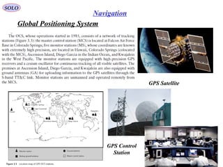
![Global Positioning System
SOLO
110
Navigation
Other satellite navigation systems in use or
various states of development include:
• GLONASS – Russia's global navigation
system. Fully operational worldwide.
• GALILEO – a global system being
developed by the European Union and other
partner countries, planned to be operational
by 2014 (and fully deployed by 2019)
• BEIDOU – People's Republic of China's
regional system, currently limited to Asia and
the West Pacific[123]
• COMPASS – People's Republic of China's
global system, planned to be operational by
2020.
• IRNSS – India's regional navigation
system, planned to be operational by 2012,
covering India and Northern Indian Ocean.
• QZSS – Japanese regional system covering
Asia and Oceania.
Comparison of GPS, GLONASS, Galileo and Compass (medium earth orbit)
satellite navigation system orbits with the International Space Station, Hubble
Space Telescope and Iridium constellation orbits, Geostationary Earth Orbit, and
the nominal size of the Earth.[121]
The Moon's orbit is around 9 times larger (in
radius and length) than geostationary orbit](https://image.slidesharecdn.com/4-navigationsystems-150812122519-lva1-app6892/85/4-navigation-systems-110-320.jpg)
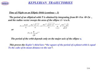
![117
SOLO KEPLERIAN TRAJECTORIES
Time of Flight on an Elliptic Orbit (continue – 4)
From
x
y
eac =
a a
( ) 2/12
1 eab −=
rΘ
FOCUS
EMPTY
FOCUS
c
→
P1
→
Q1
a
F
Q
O VS
E
P
Eeary
aeEarx
ellipse
ellipse
sin1sin
coscos
2
−=Θ=
−=Θ=
we have
( ) ( )[ ] [ ]
( )Eea
EeEeaEeaaeEar
cos1
coscos21sin1cos
2/1222/12222
−=
+−=−+−=
Therefore
Θ+
Θ−
=
−
−
=Θ
Θ+
Θ+
=
−
−
=Θ
cos1
sin1
sin
cos1
sin1
sin
cos1
cos
cos
cos1
cos
cos
22
e
e
E
Ee
Ee
e
e
E
Ee
eE
( )( )
Ee
Ee
Ee
eEEe
sin1
cos11
sin1
coscos1
sin
cos1
2
tan
22
−
−+
=
−
+−−
=
Θ
Θ−
=
Θ
From
2
tan
1
1
2
tan
E
e
e
−
+
=
Θ
or
and are always in the same quadrant.2
Θ
2
E](https://image.slidesharecdn.com/4-navigationsystems-150812122519-lva1-app6892/85/4-navigation-systems-117-320.jpg)
![GPS Broadcast Ephemerides
SOLO
120
Navigation
( )
Θ+=
=
= ωuur
ur
y
x
q ellipse
ellipse
Orbit
0
sin
cos
0
( )
2
1
0
cos
sin
0
e
an
ue
u
y
x
q ellipse
ellipse
Orbit
Orbit
−
⋅
⋅
+
−
=
=
( ) oecoec ttt ⋅+−⋅=Θ ωω
[ ] [ ] [ ]
−−Ω−=
=
0
sin
cos
0
313 ur
ur
iy
x
C
z
y
x
ellipse
ellipse
G
G
ωε
Θ+= ωu](https://image.slidesharecdn.com/4-navigationsystems-150812122519-lva1-app6892/85/4-navigation-systems-120-320.jpg)

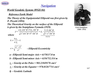
![SOLO
166
Navigation
World Geodetic System (WGS 84)
Reference Earth Model
Clairaut's theorem
Clairaut's theorem, published in 1743 by Alexis Claude Clairaut in
his Théorie de la figure de la terre, tirée des principes de
l'hydrostatique,[1]
synthesized physical and geodetic evidence that
the Earth is an oblate rotational ellipsoid. It is a general
mathematical law applying to spheroids of revolution. It was
initially used to relate the gravity at any point on the Earth's
surface to the position of that point, allowing the ellipticity of the
Earth to be calculated from measurements of gravity at different
latitudes.
Clairaut's formula for the acceleration due to gravity g on the surface of a spheroid
at latitude φ, was:
where G is the value of the acceleration of gravity at the equator, m the ratio of
the centrifugal force to gravity at the equator, and f the flattening of a meridian
section of the earth, defined as:
a
ba
f
−
=:
Alexis Claude Clairaut
)1713–1765(
−+= φ2
sin
2
5
1 fmGg](https://image.slidesharecdn.com/4-navigationsystems-150812122519-lva1-app6892/85/4-navigation-systems-166-320.jpg)
![SOLO
168
Navigation
World Geodetic System (WGS 84)
Reference Earth Model
The coordinate origin of WGS 84 is meant to be located at the
Earth's center of mass; the error is believed to be less than 2 cm.
The WGS 84 meridian of zero longitude is the IERS Reference
Meridian. 5.31 arc seconds or 102.5 meters (336.3 ft) east of the
Greenwich meridian at the latitude of the Royal Observatory.
The WGS 84 datum surface is an oblate spheroid (ellipsoid) with major
(transverse) radius a = 6378137 m at the equator and flattening
f = 1/298.257223563.The polar semi-minor (conjugate) radius b then equals a
times (1−f), or b = 6356752.3142 m.
Presently WGS 84 uses the EGM96 (Earth Gravitational Model 1996) Geoid,
revised in 2004. This Geoid defines the nominal sea level surface by means of a
spherical harmonics series of degree 360 (which provides about 100 km
horizontal resolution).[7]
The deviations of the EGM96 Geoid from the WGS 84
Reference Ellipsoid range from about −105 m to about +85 m.[8]
EGM96 differs
from the original WGS 84 Geoid, referred to as EGM84.](https://image.slidesharecdn.com/4-navigationsystems-150812122519-lva1-app6892/85/4-navigation-systems-168-320.jpg)
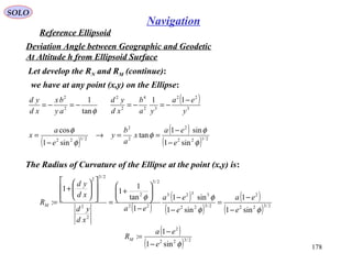
![SOLO
179
Navigation
Reference Ellipsoid
Deviation Angle between Geographic and Geodetic
At Altitude h from Ellipsoid Surface
( )
( ) 2/322
2
sin1
1
:
φe
ea
RM
−
−
=
( ) 2/122
sin1cos φφ e
ax
RN
−
==
a
ba
f
−
=: 2
2
22
2
2: ff
a
ba
e −=
−
=Using
( )
( )[ ]
( ) ( ) [ ] ++−≈
+−++−≈
−−
−
= φφ
φ
2222
2/322
2
sin321sin2
2
3
121
sin21
1
: ffaffffa
ff
fa
RM
( )[ ]
( ) [ ]φφ
φ
222
2/122
sin31sin2
2
3
1
sin21
faffa
ff
a
RN +≈
+−+≈
−−
=
[ ]φ2
sin321 ffaRM +−≈
[ ]φ2
sin31 faRN +≈
We used and we neglect f2
terms
( )
( ) +
−
++=
− !2
1
1
1
1 nn
xn
x
n](https://image.slidesharecdn.com/4-navigationsystems-150812122519-lva1-app6892/85/4-navigation-systems-179-320.jpg)
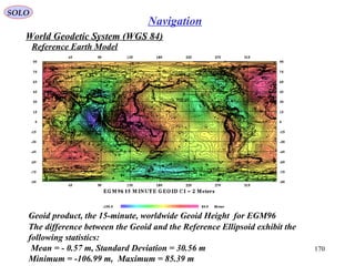
![SOLO
180
Navigation
World Geodetic System (WGS 84)
Reference Earth Model
The definition of geodetic latitude (φ) and
longitude (λ) on an ellipsoid. The normal
to the surface does not pass through the
centre
Reference Ellipsoid
Geodetic latitude: the angle between the
normal and the equatorial plane. The
standard notation in English publications is ϕ
Geocentric latitude: the equatorial plane and
the radius from the centre to a point on the
surface. The relation between the geocentric
latitude (ψ) and the geodetic latitude ( ) isϕ
derived in the above references as
The definition of geodetic (or
geographic) and geocentric latitudes
( ) ( )[ ]φφψ tan1tan 21
e−= −](https://image.slidesharecdn.com/4-navigationsystems-150812122519-lva1-app6892/85/4-navigation-systems-180-320.jpg)

The document outlines the principles of navigation systems for aircraft, detailing the various headings, tracks, and the calculation of deviations from desired flight paths using spherical trigonometry. It also explains the concept of great circles as the shortest distance between two points on Earth and introduces multiple coordinate systems relevant to navigation. Furthermore, it discusses the dynamics of air vehicles within a spherical Earth model and the forces acting on them.


![谷歌留痕技术 [ 𝙩𝙤𝙥 𝟮𝟯𝟯. 𝙘 𝙤𝙢 ]](https://cdn.slidesharecdn.com/ss_thumbnails/top233-260130174328-3833018c-thumbnail.jpg?width=640&height=640&fit=bounds)


