Downloaded 63 times
![4
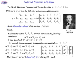
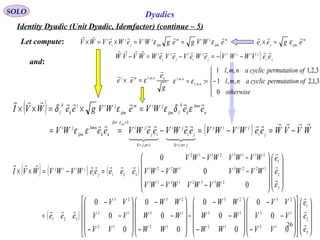
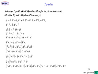
SOLO Vectors & Tensors in a 3D Space
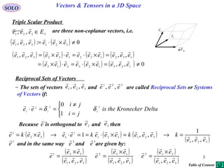
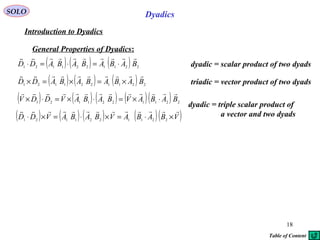
Reciprocal Sets of Vectors (continue)
By using the previous equations we get:
( ) ( )
( )
( )[ ] ( )[ ]
( ) ( )321
3
2
321
13323132
2
321
133221
,,,,,, eee
e
eee
eeeeeeee
eee
eeee
ee
=
⋅×−⋅×
=
×××
=×
( )
( )
( )
( )
( )
( )321
213
321
132
321
321
,,,,,, eee
ee
e
eee
ee
e
eee
ee
e
×
=
×
=
×
=
( ) ( )
( ) ( )
0
,,
1
,,
,,
321321
3
3321321
≠=
⋅
==⋅×
eeeeee
ee
eeeeee
Multiplying (scalar product) this equation by we get:
3
e
In the same way we can show that:
Therefore are also non-coplanar, and:
321
,, eee
( ) ( ) 1,,,, 321
321
=eeeeee
( )
( )
( )
( )
( )
( )321
21
3321
13
2321
32
1
,,,,,, eee
ee
e
eee
ee
e
eee
ee
e
×
=
×
=
×
=
1e
2e
3
e
1
e
2
e
3
e
Table of Content](https://image.slidesharecdn.com/dyadics-140928113250-phpapp01/85/Dyadics-4-320.jpg)
![10
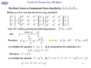
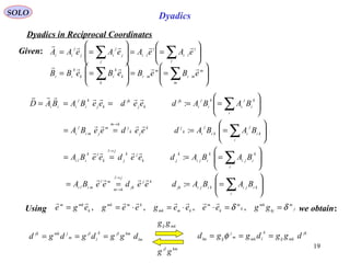
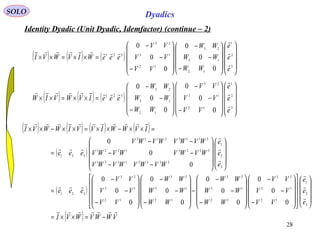
SOLO Vectors & Tensors in a 3D Space
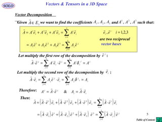
Let find the relation between g and
The Metric Tensor or Fundamental Tensor Specified by .3321 ,, Eeee ∈
( ) ( )321321 :,, eeeeee
×⋅=
We shall write the decomposition of in the vector base32 ee
× 321 ,, eee
3
3
2
2
1
1
32 eeeee
λλλ ++=×
Let find λ1
, λ2
, λ3
. Multiply the previous equation (scalar product) by .1e
( ) ( ) i
i
ggggeeeeee 113
3
12
2
11
1
321321 ,, λλλλ =++==×⋅
Multiply this equation by g1i
: ( ) ii
i
ii
ggeeeg λλ ==
1
1
1321
1
,,
Therefore: ( )321
1
,, eeeg ii
=λ
Let compute now:
( ) ( ) ( ) ( ) ( ) ( )321
1
0
323
3
0
322
2
321
1
3232
eeeeeeeeeeeeeeee
×⋅=×⋅+×⋅+×⋅=×⋅× λλλλ
( ) ( )[ ]
( )
( )[ ]
( )
( ) ( )[ ]
( ) ( ) ( ) ( )321
11
321
11
321
2
233322
321
3322332
321
3232
321
32321
,,,,,,,,
,,,,
eee
gg
eee
G
eee
ggg
eee
eeeeeee
eee
eeee
eee
eeee
==
−
=
⋅−⋅⋅
=
××⋅
=
×⋅×
=λ
From those equations we obtain:
( )321
11
1
,, eee
gg
=λ
Finally: ( ) ( ) geeeeee =⇒= 321
2
321
1
,,,,
λ
We can see that if are collinear than and g are zero.321 ,, eee
321
,, eee
Table of Content](https://image.slidesharecdn.com/dyadics-140928113250-phpapp01/85/Dyadics-10-320.jpg)
![11
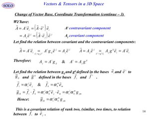
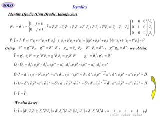
SOLO Vectors & Tensors in a 3D Space
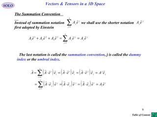
Let choose another base and its reciprocal
Change of Vector Base, Coordinate Transformation
( )321 ,, fff
( )321
,, fff
[ ]
=
=
→=
3
2
1
3
2
1
3
3
2
3
1
3
3
2
2
2
1
2
3
1
2
1
1
1
3
2
1
e
e
e
L
e
e
e
f
f
f
ef j
j
ii
ααα
ααα
ααα
α
where j
i
j
i ef
⋅=α
By tacking the inverse of those equations we obtain:
[ ]
=
=
→=
−
3
2
1
1
3
2
1
3
3
2
3
1
3
3
2
2
2
1
2
3
1
2
1
1
1
3
2
1
f
f
f
L
f
f
f
e
e
e
fe i
j
ij
βββ
βββ
βββ
β
where j
ij
i ef
⋅=β
Because are the coefficients of the inverse matrix with coefficients :
j
i
β j
i
α
i
j
i
k
k
j
δαβ =](https://image.slidesharecdn.com/dyadics-140928113250-phpapp01/85/Dyadics-11-320.jpg)
![12
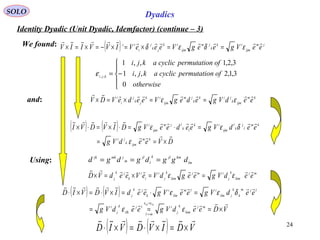
SOLO Vectors & Tensors in a 3D Space
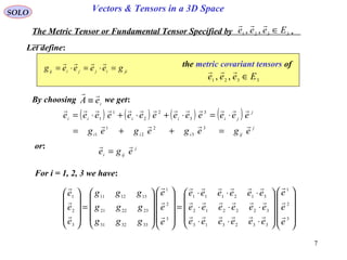
Let write any vector in those two bases:
Change of Vector Base, Coordinate Transformation (continue – 1)
A
[ ]
=
=
→
⋅=
=
3
2
1
3
2
1
3
3
2
3
1
3
3
2
2
2
1
2
3
1
2
1
1
1
3
2
1
e
e
e
L
e
e
e
f
f
f
ef
ef
ji
j
i
j
j
ii
ααα
ααα
ααα
α
α
then:
[ ]
=
=
→
⋅=
= −
3
2
1
1
3
2
1
3
3
3
2
3
1
2
3
2
2
2
1
1
3
1
2
1
1
3
2
1
E
E
E
L
E
E
E
F
F
F
ef
EF T
j
ii
j
i
j
ji
βββ
βββ
βββ
β
β
i
i
j
j
fFeEA
== iijj
fAFeAE
⋅=⋅= &
i
j
ji
i
i
j
j
j
j
i
i
EFfEeEfF ββ =→==
or:
But we remember that:
We can see that the relation between the components F1
, F2
, F3
to E1
, E2
, E3
is
not similar, contravariant, to the relation between the two bases of vectors
to . Therefore we define F1
, F2
, F3
and E1
, E2
, E3
as the contravariant
components of the bases and .
( )321 ,, fff
( )321
,, eee
( )321 ,, fff
( )321 ,, eee
where](https://image.slidesharecdn.com/dyadics-140928113250-phpapp01/85/Dyadics-12-320.jpg)
![13
SOLO Vectors & Tensors in a 3D Space
Let write now the vector in the two bases and
Change of Vector Base, Coordinate Transformation (continue – 2)
A
[ ]
=
=
→=
3
2
1
3
2
1
3
3
2
3
1
3
3
2
2
2
1
2
3
1
2
1
1
1
3
2
1
E
E
E
L
E
E
E
F
F
F
EF j
iji
ααα
ααα
ααα
α
and
i
i
j
j fFeEA
== iijj fAFeAE
⋅=⋅= &
then:
( )321
,, fff
( )321
,, eee
where
j
ij
ef
ijjjjii EfeEeEAfAF j
iji
α
α=⋅
=⋅==⋅=
We can see that the relation between the components F1, F2, F3 to E1, E2, E3 is
similar, covariant, to the relation between the two bases of vectors
to . Therefore wew define F1
, F2
, F3
and E1
, E2
, E3
as the covariant
components of the bases and .
( )321
,, fff
( )321
,, eee
( )321
,, fff
( )321
,, eee
](https://image.slidesharecdn.com/dyadics-140928113250-phpapp01/85/Dyadics-13-320.jpg)
![15
SOLO Vectors & Tensors in a 3D Space
Change of Vector Base, Coordinate Transformation (continue – 4)
[ ]
=
=
→
⋅=
=
3
2
1
3
2
1
3
3
2
3
1
3
3
2
2
2
1
2
3
1
2
1
1
1
3
2
1
e
e
e
L
e
e
e
f
f
f
ef
ef
ji
j
i
j
j
ii
ααα
ααα
ααα
α
α
Since we have:k
iki fgf
= ( ) m
jm
j
i
ege
j
j
i
ef
k
iki
egefgf m
jmjj
j
ii
αα
α ==
===
and: ( ) ( ) m
jm
j
i
km
kjm
j
i
gg
k
ik egfgfg
mjm
m
k
j
iik
ααα
αα
==
=
Therefore, by equalizing the terms that multiply we obtain:
[ ]
=
=
→=
3
2
1
3
2
1
3
3
3
2
3
1
2
3
2
2
2
1
1
3
1
2
1
1
3
2
1
f
f
f
L
f
f
f
e
e
e
fe
Tkm
k
m
ααα
ααα
ααα
α
We found the relation:
( )jm
j
i gα](https://image.slidesharecdn.com/dyadics-140928113250-phpapp01/85/Dyadics-15-320.jpg)
![16
SOLO Vectors & Tensors in a 3D Space
Change of Vector Base, Coordinate Transformation (continue – 5)
Therefore:
Let take the inverse of the relation by multiplying by and summarize on m:
j
m
β
[ ]
=
=
→= −
3
2
1
1
3
2
1
3
3
3
2
3
1
2
3
2
2
2
1
1
3
1
2
1
1
3
2
1
e
e
e
L
e
e
e
f
f
f
ef
Tmj
m
j
βββ
βββ
βββ
β
km
k
m
fe
α=
jkj
k
km
k
j
m
mj
m fffe
=== δαββ
From the relation: mk
m
kjj
i
i
efef
ββ == &
we have: jmk
m
j
i
mjk
m
j
i
kiik
geeffg ββββ =⋅=⋅=
or: jmk
m
j
i
ik
gg ββ= This is a contravariant relation of rank two.
From the relation:
m
m
kk
jj
i
i
efef
αβ == &
we have: m
j
m
k
i
jm
jm
k
i
j
i
kk
i
eeff δαβαβδ =⋅==⋅
or: This is a relation once covariant and once contravariant of
rank two.
m
j
m
k
i
j
i
k δαβδ =
Table of Content](https://image.slidesharecdn.com/dyadics-140928113250-phpapp01/85/Dyadics-16-320.jpg)
![20
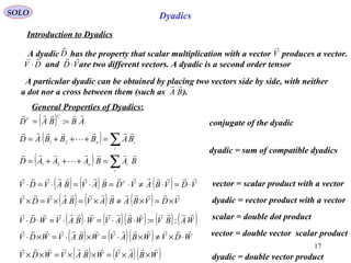
SOLO Dyadics
Dyadics in Reciprocal Coordinates
Given:
==
== ∑∑ l
l
li
l
li
j
j
j
ij
j
ii
eAeAeAeAA
==
== ∑∑ m
m
mi
m
mi
k
k
k
ik
k
ii
eBeBeBeBB
( ) ( ) [ ]
=
===
3
2
1
321
3
2
1
333231
232221
131211
321
e
e
e
Deee
e
e
e
ddd
ddd
ddd
eeeeedBAD kj
jk
ii
Decomposition of a dyadic in symmetric and anti-symmetric parts:
( ) ( ) [ ]
=
===
3
2
1
321
3
2
1
332313
322212
312111
321
e
e
e
Deee
e
e
e
ddd
ddd
ddd
eeeeedABD
T
kj
kj
ii
C
( ) ( ) ( ) ( )
( )
( ) ( ) ( )
( ) ( ) ( )
( ) ( ) ( )
[ ] [ ]( )
( )
( ) ( )
( ) ( )
( ) ( )
[ ] [ ]( )
−−−−
−−−
−−
+
+++
+++
+++
=
Ω+Φ=−++=−++=
−+
−
3
2
1
2
1
32233113
32232112
31132112
321
3
2
1
2
1
333332233113
322322222112
311321121111
321
0
0
0
2
1
2
1
2
1
2
1
2
1
2
1
e
e
e
dddd
dddd
dddd
eee
e
e
e
dddddd
dddddd
dddddd
eee
eeddeeddDDDDD
TT
DDDD
kj
kjjk
kj
kjjk
symmetricanti
C
symmetric
C
The conjugate dyadic of is:D
Table of Content](https://image.slidesharecdn.com/dyadics-140928113250-phpapp01/85/Dyadics-20-320.jpg)
![22
SOLO Dyadics
Identity Dyadic (Unit Dyadic, Idemfactor) (continue – 1)
( ) ( )
( ) ( ) ( )[ ]211231331232231
3
3
2
2
1
13
3
2
2
1
1
eeeeVeeeeVeeeeVg
eeeeeeeVeVeVIV
−+−+−=
++×++=×
( ) ( ) ( ) ( )32121
3
13
2
32
1
,,
111
eeegee
g
eee
g
eee
g
e
=×=×=×=
We found:
Using:
( ) WVWIVWIV
⋅=⋅⋅=⋅⋅VVIIV
=⋅=⋅
( ) ( )
( ) ( ) ( )[ ]211231331232231
3
3
2
2
1
1
3
3
2
2
1
1
eeeeVeeeeVeeeeVg
eVeVeVeeeeeeVI
−+−+−=
++×++=×
( )c
IVVIIV
×−=×=×
( )
( ) ( ) ( )( )
( )
−
−
−
=
−+−+−=
==×=×−=×=×
3
2
1
12
13
23
321
211231331232231
0
0
0
e
e
e
VV
VV
VV
eeeg
eeeeVeeeeVeeeeVg
eeVgeegVeeeVIVVIIV jm
ijm
ik
k
jm
ijm
ik
jk
j
i
i
c
εδεδ](https://image.slidesharecdn.com/dyadics-140928113250-phpapp01/85/Dyadics-22-320.jpg)
![23
SOLO Dyadics
Identity Dyadic (Unit Dyadic, Idemfactor) (continue – 2)
( ) ( ) ( )
−
−
−
−
−
−
−
−
−
−
−
−
−
=
−−
−−
−−
=
×⋅=×=⋅×=⋅×
⋅=×=×
3
2
1
12
13
23
12
13
23
12
13
23
12
13
23
3
2
1
23321331
32231221
31132112
0
0
0
0
0
0
0
0
0
0
0
0
0
0
0
e
e
e
VV
VV
VV
WW
WW
WW
WW
WW
WW
VV
VV
VV
g
e
e
e
WVWVWVWV
WVWVWVWV
WVWVWVWV
g
WVIWVWIVWVI
VIVIVVI
( ) ( ) ( ) ( ) ( )[ ] ( )
( ) ( ) ( )[ ]
( ) ( ) ( )[ ] WVeeWVWVeeWVWVeeWVWV
eWVWVeWVWVeWVWVg
eWeWeWeeeeVeeeeVeeeeVgWIVWVI
k
m
k
m
ee
×=×−+×−+×−=
−+−+−=
++⋅−+−+−=⋅×=⋅×
=⋅
21
1221
13
3113
32
2332
312212311312332
3
3
2
2
1
1211231331232231
δ
( ) ( ) WVWIVWVI
×=⋅×=⋅×
( ) ( ) ( ) ( )[ ]211231331232231
eeeeVeeeeVeeeeVgIVVIIV c
−+−+−=×−=×=×](https://image.slidesharecdn.com/dyadics-140928113250-phpapp01/85/Dyadics-23-320.jpg)
![25
SOLO Dyadics
Identity Dyadic (Unit Dyadic, Idemfactor) (continue – 4)
( ) ( ) ( )[ ]
( ) ( ) ( )[ ]
( ) ( ) ( )[ ]
( ) ( ) ( )[ ]
( )
( ) ( ) ( )
( ) ( ) ( )
( ) ( ) ( )
( )
−
−
−
=
−−−
−−−
−−−
=
−+−+−+
−+−+−+
−+−+−
=
−+−+−=
==×=×
3
2
1
3
3
2
3
1
3
3
2
2
2
1
2
3
1
2
1
1
1
12
13
23
321
3
2
1
3
12
3
21
2
12
2
21
1
12
1
21
3
31
3
13
2
31
2
13
1
31
1
13
3
23
3
32
2
23
2
32
1
23
1
32
321
31
3
22
3
133
3
11
3
322
3
33
3
21
21
2
22
2
133
2
11
2
322
2
33
2
21
11
1
22
1
133
1
11
1
322
1
33
1
21
122133113223321
0
0
0
e
e
e
ddd
ddd
ddd
VV
VV
VV
eeeg
e
e
e
dVdVdVdVdVdV
dVdVdVdVdVdV
dVdVdVdVdVdV
eeeg
eededVededVededV
eededVededVededV
eededVededVededV
g
eededVededVededVg
eedVgedegVeedeVDV
k
kkkkkk
km
ijmk
jik
k
jm
ijm
ik
jk
j
i
i
εε
−=
otherwise
ofnpermutatiocyclicakji
ofnpermutatiocyclicakji
kji
0
3,1,2,,1
3,2,1,,1
,,
ε](https://image.slidesharecdn.com/dyadics-140928113250-phpapp01/85/Dyadics-25-320.jpg)
![27
SOLO Dyadics
Identity Dyadic (Unit Dyadic, Idemfactor) (continue – 2)
( ) ( ) ( ) ( ) ( )[ ] ( )
( )
( ) ( ) ( )
( ) ( ) ( )
( ) ( ) ( )
( )
−
−
−
−
−
−
=
+−
+−
+−
=
++⋅×−+−+−=××=××
=×
3
2
1
12
13
23
12
13
23
321
3
2
1
2
2
1
1
3
2
3
1
2
3
3
3
1
1
2
1
1
3
1
2
3
3
2
2
321
3
3
2
2
1
1
211231331232231
0
0
0
0
0
0
,,
e
e
e
WW
WW
WW
VV
VV
VV
eee
e
e
e
WVWVWVWV
WVWVWVWV
WVWVWVWV
eee
eWeWeWeeeeVeeeeVeeeeVgWIVWVI
g
e
ee kkjiji
ε
( ) ( ) ( ) ( )[ ]211231331232231
eeeeVeeeeVeeeeVgIVVIIV c
−+−+−=×−=×=×
( ) ( ) ( ) ( ) ( ) ( )[ ]
( )
( ) ( ) ( )
( ) ( ) ( )
( ) ( ) ( )
( )
−
−
−
−
−
−
=
+−
+−
+−
=
−+−+−×++=××=××
=×
3
2
1
12
13
23
12
13
23
321
3
2
1
2
2
1
1
2
3
1
3
3
2
3
3
1
1
1
2
3
1
2
1
3
3
2
2
321
2112313312322313
3
2
2
1
1
0
0
0
0
0
0
,,
e
e
e
VV
VV
VV
WW
WW
WW
eee
e
e
e
WVWVWVWV
WVWVWVWV
WVWVWVWV
eee
eeeeVeeeeVeeeeVgeWeWeWIVWVIW
g
e
ee kkjiji
ε](https://image.slidesharecdn.com/dyadics-140928113250-phpapp01/85/Dyadics-27-320.jpg)
![30
SOLO Dyadics
Coordinate Transformation of Dyadics in Reciprocal Coordinates
kj
jkk
jk
j
k
jk
j
kj
jk
kj
k
i
j
iii eedeedeedeedeeBABAD
======
nm
mnn
mn
m
n
mn
m
nm
mn
ii ffdffdffdffdBAD
=====
where
k
jk
jk
j
n
k
j
mn
mn
mn
m
eedeedffdD
=== βα
Let find the relation between defined in the bases and to
defined in the bases and .
i
e
i
e
i
f
i
f
k
j
d
n
m
d
[ ]
=
=
→
=
= −
3
2
1
1
3
2
1
3
3
3
2
3
1
2
3
2
2
2
1
1
3
1
2
1
1
3
2
1
e
e
e
L
e
e
e
f
f
f
ef T
i
j
i
k
k
j
mj
m
j
βββ
βββ
βββ
δαβ
β
[ ]
=
=
→
⋅=
=
3
2
1
3
2
1
3
3
2
3
1
3
3
2
2
2
1
2
3
1
2
1
1
1
3
2
1
e
e
e
L
e
e
e
f
f
f
ef
ef
ji
j
i
j
j
ii
ααα
ααα
ααα
α
α
n
k
j
mn
m
k
j
dd βα=
n
mm
n
n
k
k
j
j
mn
mm
n
k
j
n
k
j
mn
mm
n
k
jk
j
dddd
m
k
k
m
===
δδ
αββααββααβ
m
j
k
nk
j
n
m
dd αβ=](https://image.slidesharecdn.com/dyadics-140928113250-phpapp01/85/Dyadics-30-320.jpg)
![31
SOLO Dyadics
Coordinate Transformation of Dyadics in Reciprocal Coordinates (continuous – 1)
where
[ ]
=
=
→
=
= −
3
2
1
1
3
2
1
3
3
3
2
3
1
2
3
2
2
2
1
1
3
1
2
1
1
3
2
1
e
e
e
L
e
e
e
f
f
f
ef T
i
j
i
k
k
j
mj
m
j
βββ
βββ
βββ
δαβ
β
[ ]
=
=
→
⋅=
=
3
2
1
3
2
1
3
3
2
3
1
3
3
2
2
2
1
2
3
1
2
1
1
1
3
2
1
e
e
e
L
e
e
e
f
f
f
ef
ef
ji
j
i
j
j
ii
ααα
ααα
ααα
α
α
m
j
k
nk
j
n
m
dd αβ=
We found
[ ]
[ ] [ ] [ ] 1
3
3
2
3
1
3
3
2
2
2
1
2
3
1
2
1
1
1
3
3
2
3
1
3
3
2
2
2
1
2
3
1
2
1
1
1
3
3
2
3
1
3
3
2
2
2
1
2
3
1
2
1
1
1
3
3
2
3
1
3
3
2
2
2
1
2
3
1
2
1
1
1
:
−
=
=
=
LDL
ddd
ddd
ddd
ddd
ddd
ddd
D
βββ
βββ
βββ
ααα
ααα
ααα
Table of Content](https://image.slidesharecdn.com/dyadics-140928113250-phpapp01/85/Dyadics-31-320.jpg)
![32
SOLO Dyadics
Dyadic Invariants
The invariants of the dyadic are derived from the following invariant equation
[ ] [ ] [ ] [ ] [ ] [ ]( ) [ ]
[ ] [ ] [ ]( ) [ ]( ) 0detdetdetdet
detdetdet
3333
1
1
1
33
1
3333
=−=−=
−=−=−
−
−−
DIDILL
LDILLDLIDI
xx
xxx
λλ
λλλ
This is the invariant characteristic equation derived from the dyadic
[ ]( )
( ) ( )[ ] ( ) ( )
( ) ( )
0
detdet
2
3
1
2
3
1
2
2
1
3
3
1
1
3
3
2
2
1
3
3
1
2
2
1
2
3
3
2
1
1
3
3
2
2
1
1
1
3
3
1
1
2
2
1
2
3
3
2
3
3
2
2
3
3
1
1
2
2
1
12
3
3
2
2
1
13
2
2
1
3
2
3
1
2
1
3
3
1
1
3
3
2
3
3
1
2
1
2
2
1
2
3
3
2
3
3
2
2
3
3
2
22
1
1
3
3
2
3
1
3
3
2
2
2
1
2
3
1
2
1
1
1
33
=−+−++−
−−−+++++−=
−+−−+−+−++−−=
−−−
−−−
−−−
=−
dddddddddddddddddd
ddddddddddddddd
ddddddddddddddddddd
ddd
ddd
ddd
DI x
λλλ
λλλλλ
λ
λ
λ
λ
We found the following three scalar invariants of the dyadic
( ) ( )
2
3
1
2
3
1
1
3
3
2
2
1
3
3
2
2
1
1
3
3
1
2
2
1
2
2
1
3
3
1
2
3
3
2
1
1
3
1
3
3
1
1
2
2
1
2
3
3
2
3
3
2
2
3
3
1
1
2
2
1
1
23
3
2
2
1
1
1
ddddddddddddddddddI
ddddddddddddIdddI
−−−++=
−−−++=++=
[ ] [ ] [ ] [ ] 1−
= LDLDWe found that under a coordinate transformation :[ ] [ ] [ ]eLf
=
Any dyadic has five important invariants associated with: three scalar invariants,
one dyadic invariant and one vector invariant.](https://image.slidesharecdn.com/dyadics-140928113250-phpapp01/85/Dyadics-32-320.jpg)
![33
SOLO Dyadics
Dyadics Invariants (continue – 1)
We found the following three scalar invariants of a dyadic
Let Compute
( ) ( ) i
k
k
i
m
k
i
m
k
i
m
ki
ji
m
k
j
m
ki
ji
m
k
j
m
i
i
mk
jk
j
ddddddeeeeddeedeedDD ===⋅⋅== δδδ
::
( ) [ ] SDDscalarDtracedddI
===++= 3
3
2
2
1
1
1
( )1
3
3
1
1
2
2
1
2
3
3
2
3
3
2
2
3
3
1
1
2
2
1
1
2
ddddddddddddI −−−++=
[ ]DddddddddddddddddddI det2
3
1
2
3
1
1
3
3
2
2
1
3
3
2
2
1
1
3
3
1
2
2
1
2
2
1
3
3
1
2
3
3
2
1
1
3
=−−−++=
The matrix [ ]
=
333231
232221
131211
ddd
ddd
ddd
D
[ ]
−
−−
−
=
2221
1211
2321
1311
2322
1312
3231
1211
3331
1311
3332
1312
3231
2221
3331
2321
3332
2322
:
dd
dd
dd
dd
dd
dd
dd
dd
dd
dd
dd
dd
dd
dd
dd
dd
dd
dd
D adj
The adjoin dyadic is defined as
( ) [ ]
=
3
2
1
321
:
e
e
e
DeeeD adjadj
( ) [ ]
=
3
2
1
321:
e
e
e
DeeeD
The adjoin dyadic is the fourth
dyadic invariant.D
adj
D
](https://image.slidesharecdn.com/dyadics-140928113250-phpapp01/85/Dyadics-33-320.jpg)
![34
SOLO Dyadics
Dyadics Invariants (continue – 2)
We have:
If we can define:
and
[ ] [ ] [ ][ ] 33det xadj IDDD =
[ ] 0det 3 ≠= ID [ ] [ ] [ ] [ ] [ ] [ ] 33
11
det/: xadj IDDDDD =→=
−−
( ) [ ]
=
−−
3
2
1
1
321
1
:
e
e
e
DeeeD
( ) [ ] ( ) [ ] ( ) [ ] I
e
e
e
Ieee
e
e
e
Deee
e
e
e
DeeeDD x
=
=
=⋅
−−
3
2
1
33321
3
2
1
1
321
3
2
1
321
1](https://image.slidesharecdn.com/dyadics-140928113250-phpapp01/85/Dyadics-34-320.jpg)
![35
SOLO Dyadics
Dyadics Invariants (continue – 3)
The fifth dyadic invariant is the vector obtained by introducing the cross vector
product between the dyadic vectors
kj
jkk
jk
j
k
jk
j
kj
jk
kj
k
i
j
iii eedeedeedeedeeBABAD
======
kj
jkk
jk
j
k
jk
j
kj
jk
kj
k
i
j
iiiV
eedeedeedeedeeBABAD
×=×=×=×=×=×=
( ) ( )321 ,, eeegee
g
e kj
ijki
=×=
ε
Use
( ) ( ) ( )[ ]321122133113223
eddeddeddgedgD ijk
ijkV
−+−+−== ε
We defined the decomposition of a dyadic in symmetric and anti-symmetric parts:
( ) ( ) ( )
( ) ( ) ( )
( ) ( ) ( )
( ) ( ) ( )
( )
( ) ( )
( ) ( )
( ) ( )
−−−−
−−−
−−
+
+++
+++
+++
=−++=
−
ΩΦ
3
2
1
32233113
32232112
31132112
321
3
2
1
333332233113
322322222112
311321121111
321
0
0
0
2
1
2
1
2
1
2
1
e
e
e
dddd
dddd
dddd
eee
e
e
e
dddddd
dddddd
dddddd
eeeDDDDD
symmetricanti
C
symmetric
C
Since the matrix representation of the vector cross-product of isV
D
( )
( )
( )
( ) ( )
( ) ( )
( ) ( )
−−−
−−−
−−−
=×
−
−
−
=×
0
0
0
32231331
32232112
13312112
2112
1331
3223
dddd
dddd
dddd
g
dd
dd
dd
gDV
i.e. the
antisymmetric
part of
multiplied by
D
g
Table of Content](https://image.slidesharecdn.com/dyadics-140928113250-phpapp01/85/Dyadics-35-320.jpg)
![36
SOLO
Accordingly we can classify the dyadics as follows:
Dyadics
Classification of Dyadics
Physically, dyadics describe at each point the properties of the field that relate an
input or cause vector to an output or effect vector. If the family of input vectors includes
all magnitudes and directions, then one class of dyadics produces families of output
vectors that also include all magnitudes and directions. Dyadics of this class are called
“complete”. All others are called “incomplete”.
[ ] 0det 3
≠= IDIf
CompleteThe three rows/columns of
[D] are linearly independent
Property Comment Classification
[ ] 0&0det 3
≠== adj
DIDIf PlanarOnly two rows/columns of
[D] are linearly independent
LinearThe three rows/columns of
[D] are linearly dependent
If [ ] 0&0det 3
=== adjDID
A Planar Dyadic can be reduced by a suitable coordinate transformation to the
sum of two dyads (no less) 2211 BABAD
+=
A Linear Dyadic can be reduced by a suitable coordinate transformation to
a single dyad 11BAD
= Table of Content](https://image.slidesharecdn.com/dyadics-140928113250-phpapp01/85/Dyadics-36-320.jpg)
![37
SOLO Dyadics
Differentiation of Dyadics
Define:
( )tD
Suppose we have a dyadics and the vector that are differentiable
functions of the parameter scalar t.
( )tV
( ) ( ) ( ) ( ) ( ) ( )[ ] ( ) ( ) ( ) ( ) ( )[ ] ( )tVtBtAtVtDtWtBtAtVtDtVtU
⋅=⋅=⋅=⋅= :&:
( ) td
Dd
VD
td
Vd
td
Bd
AVB
td
Ad
VBA
td
Vd
td
Ud
⋅+⋅=
⋅+
⋅+⋅=
where:
+
=
td
Bd
AB
td
Ad
td
Dd
:
( ) V
td
Dd
td
Vd
DV
td
Bd
AVB
td
Ad
td
Vd
BA
td
Wd
⋅+⋅=⋅
+⋅
+⋅=
( ) ( ) V
td
Dd
td
Vd
DVD
td
d
td
Dd
VD
td
Vd
DV
td
d
⋅+⋅=⋅⋅+⋅=⋅ &
( ) ( ) V
td
Dd
td
Vd
DVD
td
d
td
Dd
VD
td
Vd
DV
td
d
×+×=××+×=× &
In the same way:](https://image.slidesharecdn.com/dyadics-140928113250-phpapp01/85/Dyadics-37-320.jpg)
![38
SOLO Dyadics
Differentiation of Dyadics
( )zyxV ,,
Gradient of a Vector .
( ) [ ]
∂
∂
∂
∂
∂
∂
∂
∂
∂
∂
∂
∂
∂
∂
∂
∂
∂
∂
=++
∂
∂
+
∂
∂
+
∂
∂
=∇
z
y
x
z
V
z
V
z
V
y
V
y
V
y
V
x
V
x
V
x
V
zyxzVyVxV
z
z
y
y
x
xV
zyx
zyx
zyx
zyx
1
1
1
111111111
This id a dyadic.
Let compute:
( ) ( ) [ ]
∂
∂
∂
∂
∂
∂
∂
∂
∂
∂
∂
∂
∂
∂
∂
∂
∂
∂
=
∂
∂
+
∂
∂
+
∂
∂
++=∇
z
y
x
z
V
y
V
x
V
z
V
y
V
x
V
z
V
y
V
x
V
zyx
z
z
y
y
x
xzVyVxVV
zyx
zyx
zyx
zyx
c
1
1
1
111111111
](https://image.slidesharecdn.com/dyadics-140928113250-phpapp01/85/Dyadics-38-320.jpg)
![39
SOLO Dyadics
Differentiation of Dyadics
( )zyxV ,,
Gradient of a Vector (continue – 1) .
( )[ ] ( )[ ]
[ ]
[ ]
∂
∂
∂
∂
−
∂
∂
−
∂
∂
−
∂
∂
−
∂
∂
−
∂
∂
+
∂
∂
−
∂
∂
−
∂
∂
−
∂
∂
+
∂
∂
−
∂
∂
+
+
∂
∂
∂
∂
+
∂
∂
∂
∂
+
∂
∂
∂
∂
+
∂
∂
∂
∂
∂
∂
+
∂
∂
∂
∂
+
∂
∂
∂
∂
+
∂
∂
∂
∂
=
∇−∇+∇+∇=∇
z
y
x
z
V
z
V
y
V
z
V
x
V
z
V
y
V
y
V
x
V
z
V
x
V
y
V
x
V
zyx
z
y
x
z
V
z
V
y
V
z
V
x
V
z
V
y
V
y
V
y
V
x
V
z
V
x
V
y
V
x
V
x
V
zyx
VVVVV
zyzxz
yzxy
xzxy
zyzxz
yzyxy
xzxyx
CC
1
1
1
2
1
2
1
2
1
0
2
1
2
1
2
1
0
111
1
1
1
2
1
2
1
2
1
2
1
2
1
2
1
111
2
1
2
1
Let decompose the gradient of the vector in the symmetric and anti-symmetric parts.](https://image.slidesharecdn.com/dyadics-140928113250-phpapp01/85/Dyadics-39-320.jpg)
![40
SOLO Dyadics
Differentiation of Dyadics
( )zyxV ,,
Gradient of a Vector (continue – 2)
Let find the scalar and vector invariants of [ ]
∂
∂
∂
∂
∂
∂
∂
∂
∂
∂
∂
∂
∂
∂
∂
∂
∂
∂
=∇
z
y
x
z
V
z
V
z
V
y
V
y
V
y
V
x
V
x
V
x
V
zyxV
zyx
zyx
zyx
1
1
1
111
( ) [ ]
∂
∂
∂
∂
∂
∂
∂
∂
∂
∂
∂
∂
∂
∂
∂
∂
∂
∂
=∇
z
y
x
z
V
y
V
x
V
z
V
y
V
x
V
z
V
y
V
x
V
zyxV
zyx
zyx
zyx
c
1
1
1
111
[ ] ( )[ ] V
z
V
y
V
x
V
VV zyx
S
c
S
⋅∇=
∂
∂
+
∂
∂
+
∂
∂
=∇=∇ Divergence of V
[ ]
V
z
z
V
y
V
y
x
V
z
V
x
y
V
x
V
V
yzzxxy
V
×∇=
∂
∂
−
∂
∂
+
∂
∂
−
∂
∂
+
∂
∂
−
∂
∂
=∇ 111
( )[ ]
∂
∂
∂
∂
−
∂
∂
−
∂
∂
−
∂
∂
−
∂
∂
−
∂
∂
+
∂
∂
−
∂
∂
−
∂
∂
−
∂
∂
+
∂
∂
−
∂
∂
+
=∇−∇
z
V
z
V
y
V
z
V
x
V
z
V
y
V
y
V
x
V
z
V
x
V
y
V
x
V
VV
zyzxz
yzxy
xzxy
c
2
1
2
1
2
1
0
2
1
2
1
2
1
0
2
1
( )[ ]
V
z
z
V
y
V
y
x
V
z
V
x
y
V
x
V
V
yzzxxy
V
c
×∇−=
∂
∂
−
∂
∂
−
∂
∂
−
∂
∂
−
∂
∂
−
∂
∂
−=∇ 111
Rotor of V
](https://image.slidesharecdn.com/dyadics-140928113250-phpapp01/85/Dyadics-40-320.jpg)
![41
Vector AnalysisSOLO
Dyadic Identities Summary
( ) ( ) ( ) CbaCabCba
⋅×=×⋅−=×⋅
( ) ( ) ( )CbaCabCba
⋅−×⋅=××
( ) CCC
⋅∇+⋅∇=⋅∇ φφφ
( ) CCC
×∇+×∇=×∇ φφφ
( ) ( ) CCC
2
∇−⋅∇∇=×∇×∇
0=×∇⋅∇ C
aCCa T
⋅=⋅
[ ]TT
aCCa
×−=×
( ) ( ) BCaBaC
TT
⋅×−=×⋅](https://image.slidesharecdn.com/dyadics-140928113250-phpapp01/85/Dyadics-41-320.jpg)
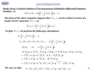
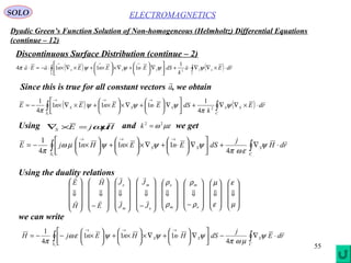
![45
Dyadic Green’s Function Solution of Non-homogeneous (Helmholtz) Differential Equations
(continue – 3)
ELECTROMAGNETICSSOLO
Using the Second Vector Green Identity
( )( )( ) ( ) ( )( )[ ] ( ) ( ) ( )( )[ ]∫∫
→
⋅⋅×∇×−×∇×⋅=×∇×∇⋅⋅−⋅×∇×∇⋅=
S
SS
V
SSSSV dSnaGEEaGdVEaGaGEI 1
where is an arbitrary constant vectora
iS
nS
n
i
iSS
1=
=dV
dSn
→
1
V
Fr
Sr
F
0r
SF rrr
−= iS
nS
dV
dSn
→
1
V
Fr
Sr
F
0r SF rrr
−=
We have
and we get
( ) ( )( )aGaG SS
consta
SS
⋅×∇×∇=⋅×∇×∇
=
( )( )( ) ( ) ( )( )[ ]
( )[ ] ( ) [ ]{ }
( ) ( )[ ]dVJJjGaaE
dVJJjEkGarraaGkE
EaGaGEI
V
mSe
V
mSeSF
V
SSSSV
∫
∫
∫
×∇+⋅⋅+⋅=
×∇−−⋅⋅−−+⋅⋅=
×∇×∇⋅⋅−⋅×∇×∇⋅=
ωµπ
ωµδπ
4
4 22
We used the fact that, since the sources and the observation point are both
in the volume V,
Sr
Fr
( ) aEdVrraE
V
SF
⋅=−⋅∫ δ
( )[ ] ( ) ( ) ( )( )[ ]∫∫ ⋅×∇×−×∇×⋅⋅+
×∇+⋅⋅−=⋅
→
S
SS
V
mSe dSaGEEaGndVJJjGaEa
14 ωµπ
Therefore we obtain
Solution of the equation: ( ) mSeSS JJjEkE ×∇−−=−×∇×∇ ωµ2](https://image.slidesharecdn.com/dyadics-140928113250-phpapp01/85/Dyadics-45-320.jpg)
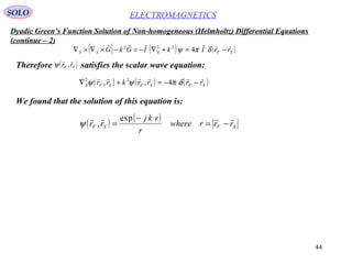
![46
Dyadic Green’s Function Solution of Non-homogeneous (Helmholtz) Differential Equations
(continue – 4)
ELECTROMAGNETICSSOLO
Let develop now the expression
( )[ ] ( ) ( ) ( )( )[ ]∫∫ ⋅×∇×−×∇×⋅⋅+
×∇+⋅⋅−=⋅
→
S
SS
V
mSe dSaGEEaGndVJJjGaEa
14 ωµπ
Solution of the equation: ( ) mSeSS JJjEkE ×∇−−=−×∇×∇ ωµ2
(continue – 1)
( ) ( ) ( )( )[ ]aGEEaGn SS
⋅×∇×−×∇×⋅⋅
→
1
( ) ( ) ( )
a
k
aa
k
aaaG
S
consta
SSSS
consta
SSSS
×∇=
=∇×∇∇⋅+×∇=
∇∇⋅+×∇=⋅×∇
→
→
=
=
ψ
ψψψ 2
0
2
11
and
( )( ) ( ) ( )
( ) aEnaEn
aEnnaEnaGE
SS
SSS
⋅∇×
×=×∇⋅
×=
=×∇×⋅=⋅×∇×=⋅⋅×∇×
→→
→→→
ψψ
ψψ
11
111](https://image.slidesharecdn.com/dyadics-140928113250-phpapp01/85/Dyadics-46-320.jpg)
![47
Dyadic Green’s Function Solution of Non-homogeneous (Helmholtz) Differential Equations
(continue – 5)
ELECTROMAGNETICSSOLO
Solution of the equation: ( ) mSeSS JJjEkE ×∇−−=−×∇×∇ ωµ2
(continue – 2)
Since is symmetric andG
k
IG SS
,
1
2
ψ
∇∇+= GaaG
⋅=⋅
( ) ( ) ( ) ( ) ( ) ( )
( ) ( )
( ) ( ) ( )Ena
k
Ena
En
k
IaEnGa
nEGanEaGnEaG
SSSS
SSSS
SSS
×∇×⋅∇∇⋅−×∇×⋅−=
×∇×⋅
∇∇+⋅−=
×∇×⋅⋅−=
××∇⋅⋅=××∇⋅⋅=⋅×∇×⋅
→→
→→
→→→
1
1
1
1
1
1
111
2
2
ψψ
ψ
( ) ( ) ( )
( ) ( ) ( ) ( ) addEna
k
Ena
k
subtractEna
k
Ena
SSSSSS
SSSS
←×∇×∇⋅∇⋅+×∇×⋅∇∇⋅−
←×∇×∇⋅∇⋅−×∇×⋅−=
→→
→→
1
1
1
1
1
1
1
22
2
ψψ
ψψ
But since ( ) ( ) ⇒=∇⋅∇=×∇×∇⇒==∇×∇
→
0&0 aaconsta SSSSSS
ψψψ
( ) ( ) ( ) ( ) ( )
( ) ψ
ψψψψψ
SS
SSSSSSSSSS
a
aaaaa
∇∇⋅=
∇⋅∇+∇∇⋅+×∇×∇+∇×∇×=∇⋅∇
we can develop the following expression
( ) ( ) ( ) ( )
( ) ( ) ( ) ( )
→→
→→
⋅×∇×∇∇⋅+××∇⋅∇⋅∇=
×∇×∇⋅∇⋅+×∇×⋅∇∇⋅−
nEa
k
nEa
k
Ena
k
Ena
k
SSSSSS
SSSSSS
1
1
1
1
1
1
1
1
22
22
ψψ
ψψ
( ) ( ) ( ) ( )[ ]
( ) ( )[ ]
→
→
⋅×∇∇⋅×∇=
⋅×∇×∇∇⋅+×∇×∇⋅∇=
nEa
k
nEaEa
k
SSS
SSSSSS
1
1
1
1
2
2
ψ
ψψ
](https://image.slidesharecdn.com/dyadics-140928113250-phpapp01/85/Dyadics-47-320.jpg)
![48
Dyadic Green’s Function Solution of Non-homogeneous (Helmholtz) Differential Equations
(continue – 6)
ELECTROMAGNETICSSOLO
Solution of the equation: ( ) mSeSS JJjEkE ×∇−−=−×∇×∇ ωµ2
(continue – 3)
We get therefore
( ) ( ) =⋅×∇×⋅
→
nEaG S 1
( ) ( ) ( )
( ) ( ) ( ) ( )Ena
k
Ena
k
Ena
k
Ena
SSSSSS
SSSS
×∇×∇⋅∇⋅+×∇×⋅∇∇⋅−
×∇×∇⋅∇⋅−×∇×⋅−=
→→
→→
1
1
1
1
1
1
1
22
2
ψψ
ψψ
( ) ( ) ( )Ena
k
Ena SSSS ×∇×∇⋅∇⋅−×∇×⋅−=
→→
1
1
1 2
ψψ
( ) ( )[ ]
→
⋅×∇∇⋅×∇+ nEa
k
SSS 1
1
2
ψ
( )( ) aEnnaGE SS
⋅∇×
×=⋅⋅×∇×
→→
ψ11We found that
therefore ( ) ( ) ( )( )[ ]aGEEaGn SS
⋅×∇×−×∇×⋅⋅
→
1
( ) ( ) ( )Ena
k
Ena SSSS
×∇×∇⋅∇⋅−×∇×⋅−=
→→
1
1
1 2
ψψ
( ) ( )[ ] aEnnEa
k
SSSS
⋅∇×
×−⋅×∇∇⋅×∇+
→→
ψψ 11
1
2
( ) ( )
×∇×∇⋅∇+∇×
×+×∇×⋅−=
→→→
En
k
EnEna SSSSS 1
1
11 2
ψψψ
( ) ( )[ ]
→
⋅×∇∇⋅×∇+ nEa
k
SSS 1
1
2
ψ
](https://image.slidesharecdn.com/dyadics-140928113250-phpapp01/85/Dyadics-48-320.jpg)
![49
Dyadic Green’s Function Solution of Non-homogeneous (Helmholtz) Differential Equations
(continue – 7)
ELECTROMAGNETICSSOLO
Solution of the equation: ( ) mSeSS JJjEkE ×∇−−=−×∇×∇ ωµ2
(continue – 4)
Since and we
get
( ) ( ) ( )( )[ ]aGEEaGn SS
⋅×∇×−×∇×⋅⋅
→
1 ( ) ( )
×∇×∇⋅∇+∇×
×+×∇×⋅−=
→→→
En
k
EnEna SSSSS 1
1
11 2
ψψψ
( ) ( )[ ]
→
⋅×∇∇⋅×∇+ nEa
k
SSS 1
1
2
ψ
( ) mSeSS JJjEkE ×∇−−=−×∇×∇ ωµ2
µεω 22
=k
( ) ( ) ( )( )[ ]
( ) ( )
( ) ( )[ ]
→
→→→→
→
⋅×∇∇⋅×∇+
∇
×∇+⋅−∇
⋅+∇×
×+×∇×⋅−=
⋅×∇×−×∇×⋅⋅
nEa
k
k
JJjnEnEnEna
aGEEaGn
SSS
S
mSeSSS
SS
1
1
1111
1
2
2
ψ
ψ
ωµψψψ
](https://image.slidesharecdn.com/dyadics-140928113250-phpapp01/85/Dyadics-49-320.jpg)
![50
Dyadic Green’s Function Solution of Non-homogeneous (Helmholtz) Differential Equations
(continue – 8)
ELECTROMAGNETICSSOLO
Solution of the equation: ( ) mSeSS JJjEkE ×∇−−=−×∇×∇ ωµ2
(continue – 5)
Let compute
( ) ( ) ( )( )[ ]∫
→
⋅⋅×∇×−×∇×⋅
S
SS dSnaGEEaG 1
( ) ( )∫
∇
×∇+⋅−∇
⋅+∇×
×+×∇×⋅−=
→→→→
S
S
mSeSSS dS
k
JJjnEnEnEna 2
1111
ψ
ωµψψψ
( ) ( )[ ] dSnEa
k S
SSS∫
→
⋅×∇∇⋅×∇+ 1
1
2
ψ
In our case the integral is performed over a closed surface S and therefore the last
integral is (using Gauss’ 5 Theorem: ):∫∫ ×∇=×
→
VS
dvAdSAn
1
( ) ( )[ ] ( ) ( )[ ] ( ) ( )[ ] 011
0
5
=×∇∇⋅⋅∇×∇=××∇∇⋅⋅∇=⋅×∇∇⋅×∇ ∫∫∫
→→
V
SSSS
Gauss
S
SSS
S
SSS dvEadSnEadSnEa
ψψψ
Compute (using Gauss’ 4 Theorem: ):( )[ ]∫∫ ⋅∇+∇⋅=
⋅
→
VS
dvABBAdSnAB
1
( )
( )
( ) ∫∫
∫∫
∫
∇⋅+
∇∇
×∇+⋅=
×∇⋅∇+⋅∇
∇
⋅+
∇∇
×∇+⋅=
×∇+⋅
∇
⋅
=
−
→
V
S
e
V
SS
mSe
k
V
mSS
j
S
S
V
SS
mSe
Gauss
S
mSe
S
dvadv
k
JJja
dvJJj
k
adv
k
JJja
dSJJjn
k
a
e
ψ
ε
ρψ
ωµ
ωµ
ψψ
ωµ
ωµ
ψ
µεω
ρω
2
0
22
4
2
2
1](https://image.slidesharecdn.com/dyadics-140928113250-phpapp01/85/Dyadics-50-320.jpg)
![51
Dyadic Green’s Function Solution of Non-homogeneous (Helmholtz) Differential Equations
(continue – 8)
ELECTROMAGNETICSSOLO
Solution of the equation: ( ) mSeSS JJjEkE ×∇−−=−×∇×∇ ωµ2
(continue – 5)
Let substitute this result in
( ) ( ) ∫∫∫ ∇⋅+
∇∇
×∇+⋅=
×∇+⋅
∇
⋅
→
V
S
e
V
SS
mSe
S
mSe
S
dvadv
k
JJjadSJJjn
k
a ψ
ε
ρψ
ωµωµ
ψ
22
1
( )[ ] ( ) ( ) ( )( )[ ]∫∫
→
⋅⋅×∇×−×∇×⋅+
×∇+⋅⋅−=⋅
S
SS
V
mSe dSnaGEEaGdVJJjGaEa 14
ωµπ
( )
×∇+⋅
∇∇
+⋅−=⋅ ∫ dVJJj
k
IaEa
V
mSe
SS
ωµψπ 2
4
( )∫
∇
⋅+∇×
×+×∇×⋅−
→→→
S
SSS dSEnEnEna ψψψ 111
( ) ∫∫ ∇⋅+
∇∇
×∇+⋅+
V
S
e
V
SS
mSe dvadv
k
JJja ψ
ε
ρψ
ωµ
2
we obtain
Since this is true for all constant vectors , after simplification and rearranging terms,
we obtain
a
( )∫∫
∇
⋅+∇×
×+×∇×−
∇−×∇+−=
→→→
S
SSS
V
S
e
mSe dSEnEnEndVJJjE ψψψ
π
ψ
ε
ρ
ψψωµ
π
111
4
1
4
1](https://image.slidesharecdn.com/dyadics-140928113250-phpapp01/85/Dyadics-51-320.jpg)
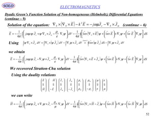
![54
Dyadic Green’s Function Solution of Non-homogeneous (Helmholtz) Differential Equations
(continue – 11)
ELECTROMAGNETICSSOLO
Discontinuous Surface Distribution (continue – 1)
Let return to
( ) ( ) ( )( )[ ]
( ) ( ) ( )( )[ ]∫
∫∫
⋅×∇×−×∇×⋅⋅=
⋅×∇×−×∇×⋅⋅+
×∇+⋅⋅−=⋅
→
+
→
1
21
1
14
00
S
SS
SS
SS
V
mSe
dSaGEEaGn
dSaGEEaGndVJJjGaEa
ωµπ
We found ( ) ( ) ( )( )[ ]
( )
( ) ( )[ ]
→
→→→→
→
⋅×∇∇⋅×∇+
∇
×∇+⋅−∇
⋅+∇×
×+×∇×⋅−=
⋅⋅×∇×−×∇×⋅
nEa
k
k
JJjnEnEnEna
naGEEaG
SSS
S
mSeSSS
SS
1
1
1111
1
2
2
00
ψ
ψ
ωµψψψ
Using Stokes’ Theorem: we have∫∫ ⋅=⋅×∇
CS
rdASdA
( ) ( )[ ] ( ) ( )∫∫∫ ⋅×∇∇⋅=⋅×∇∇⋅=⋅×∇∇⋅×∇
→
C
SS
C
SS
Stokes
S
SSS rdEardEadSnEa
ψψψ
1
1
Therefore
( ) ( ) ( )( )[ ]
( ) ( )∫∫
∫
⋅×∇∇⋅+
∇
⋅+∇×
×+×∇×⋅−=
⋅×∇×−×∇×⋅⋅=⋅
→→→
→
C
SS
S
SSS
S
SS
rdEa
k
dSEnEnEna
dSaGEEaGnEa
ψψψψ
π
2
1
111
14
1
1](https://image.slidesharecdn.com/dyadics-140928113250-phpapp01/85/Dyadics-54-320.jpg)
![56
SOLO
References
[1] Vavra, M.H., “Aero-Thermodynamics and Flow Turbomachines”,
John Wiley & Sons, 1960
Appendix B: ”Introduction to Operations Involving Dyadics”, pp.531-557
Dyadics
[2] Reddy, J.N. & Rasmussen, M.L., “Advanced Engineering Analysis”,
John Wiley & Sons, 1982, Ch. 1.5: Dyadics and Tensors, pp.107-152
[3] Chou, P.C., Pagano, N.J., “Elasticity - Tensor, Dyadic and Engineering Approaches”,
Dover, 1992, Ch. 11: Vector and Dyadic Notation in Elasticity, pp.225-244
[4] Chen-To Tai, “Dyadic Green Functions in Electromagnetic Theory”, 2nd
Ed.,
IEEE Press, 1993](https://image.slidesharecdn.com/dyadics-140928113250-phpapp01/85/Dyadics-56-320.jpg)


This document discusses vectors and tensors in three dimensions. It defines reciprocal sets of vectors, which satisfy certain orthogonality properties. It introduces the metric tensor or fundamental tensor, which is specified by three non-coplanar vectors. It proves that the determinant of the metric tensor, known as the Gram determinant, is non-zero using properties of the defining vectors.


](https://cdn.slidesharecdn.com/ss_thumbnails/virtualworkmodifiedcompatibilitymode1-160126134241-thumbnail.jpg?width=640&height=640&fit=bounds)