FITTED OPERATOR FINITE DIFFERENCE METHOD FOR SINGULARLY PERTURBED PARABOLIC CONVECTION-DIFFUSION TYPE

Informatics Engineering, an International Journal (IEIJ), Vol.5, No.1, March 2021
DOI : 10.5121/ieij.2021.5101 1
FITTED OPERATOR FINITE DIFFERENCE METHOD
FOR SINGULARLY PERTURBED PARABOLIC
CONVECTION-DIFFUSION TYPE
Tesfaye Aga Bullo and Gemechis File Duressa
Department of Mathematics, College of Natural Science, Jimma University, Jimma, P.O.
Box 378, Ethiopia
ABSTRACT
In this paper, we study the numerical solution of singularly perturbed parabolic convection-diffusion type
with boundary layers at the right side. To solve this problem, the backward-Euler with Richardson
extrapolation method is applied on the time direction and the fitted operator finite difference method on the
spatial direction is used, on the uniform grids. The stability and consistency of the method were established
very well to guarantee the convergence of the method. Numerical experimentation is carried out on model
examples, and the results are presented both in tables and graphs. Further, the present method gives a more
accurate solution than some existing methods reported in the literature.
KEYWORDS
Singularly perturbation; convection-diffusion; boundary layer; Richardson extrapolation; fitted operator.
1. INTRODUCTION
Singularly perturbed parabolic partial differential equations are types of the differential equations
whose highest order derivative multiplied by small positive parameter. Basic application of these
equations are in the Navier stoke’s equations, in modeling and analysis of heat and mass transfer
process when the thermal conductivity and diffusion coefficients are small and the rate of reaction
is large [6, 11]. The presence of a small parameter in the given differential equation leads to
difficulty to obtain satisfactory numerical solutions. Thus, numerical treatment of the singularly
perturbed parabolic initial-boundary value problem is problematic because of the presence of
boundary layers in its solution. Hence, time-dependent convection-diffusion problems have been
largely discovered by researchers. Wherever they either use time discretization followed by the
spatial discretization or discretizes all the variables at once.
Researchers like, Clavero et al. [2] used the classical implicit Euler to discretize the time variable
and the upwind scheme on a non-uniform mesh for the spatial variable. The scheme was shown to
be first-order accurate. To get a higher-order method, Kadalbajoo and Awasthi [9] used the Crank
Nicolson finite difference method to discretize the time variable along with the classical finite
difference method on a piecewise uniform mesh for the space variable. Gowrisankar and Natesan
[13] working the backward Euler to discretize the time variable and the classical upwind finite
difference method on a layer adapted mesh for the space variable. To hypothesis the mesh, the
authors used equidistribution of a positive monitor function which is a linear combination of a
constant and the second-order spatial derivative of the singular component of the solution at each
time level. Their analysis provided a first-order accuracy in time and almost first-order accuracy in

2
space. Again, Growsiankor and Natesan [12] again constructed a layer adapted mesh together with
the classical upwind finite difference method to discretize the spatial variable.
In [9], Kadalbajoo et al. used the B-spline collocation method on a piecewise uniform mesh to
discretize the spatial variable and the classical implicit Euler for time variable to obtain a higher-
order accuracy in space. Natesan and Mukherjee [8] working using the Richardson extrapolation
method to post-process a uniformly convergent method to a second-order accuracy in both
variables. But, these methods mostly treated the stated problem for small order of convergence.
Thus, it is necessary to improve the accuracy with higher order of convergence for solving
singularly perturbed parabolic convection-diffusion types.
2. FORMULATION OF NUMERICAL METHOD
Consider the singularly perturbed parabolic initial-boundary value problems of the form
2
2
( , ) ( , ) ( , ) ( , ) ( , ) ( , ) ( , )
u u u
x t x t a x t x t b x t u x t f x t
t x x
  
   
   (1)
( , ) : (0,1) (0, ]
x t T
  
subject to the initial and boundary conditions:
 
 
 
0 0
1 1
( ,0) ( ) on : ( ,0): 0 1
(0, ) ( ) on : (0, ): 0
(1, ) ( ), on : (1, ): 0
x
u x s x S x x
u t q t S t t T
u t q t S t t T
   
   
   
(2)
where  is a perturbation parameter that satisfy 0 1
   . Functions ( , )
a x t , ( , )
b x t and
( , )
f x t are assumed to be sufficiently smooth functions on the given domain  such that for the
constants  and  .
( , ) 0,
( , ) 0.
a x t
b x t
  
   (3)
Under sufficient smoothness and compatibility conditions imposed on the functions
0 1
( ), ( ), ( )
s x q t q t and ( , )
f x t , the initial-boundary value problem admits a unique solution
( , )
u x t to the assumed condition in Eq. (3), ( , ) 0
a x t  which exhibits a boundary layer of width
( )
O  near the boundary 1
x  of the domain , [8].
Consider Eq. (1) on a particular domain ( , ) : (0,1) (0,1]
x t    with the conditions in Eq. (2)
and let and
M N be positive integers. When working on  , we use a rectangular grid
k
h

whose
nodes are
 
,
m n
x t
for 0,1, . . .
m M
 and 0,1, . . .
n N
 . Here, 0 1
0 . . . 1
M
x x x
     and
0 1
0 . . . 1
N
t t t
     such grids are called tensor-product grids.

3
1 1
, , 0,1,2, . . . , and , , 0,1,2, . . . ,
n m
t nk k n N x mh h m M
N M
     
(4)
Let denote the approximate solution ( , )
n
m m n
u u x t
 at an arbitrary point( , )
m n
x t . Then,
considering the uniform discretization formula given in Eq. (4) in the t direction only, we have
the finite difference approximation for the derivatives with respect to t as:
1
1 1
2
2
( ) ( )
( ) ( ) ...
2
n
n n n
u u u u
x x k
x x
t k t

 
 

  
  (5)
Substituting Eq. (5) into Eq. (1) transforms the singularly perturbed partial differential equation to
ordinary differential equation at each ( 1)th
n  level of the form:
1 1
2
1
1 1 1
1
2
1 ( )
( ) ( ) ( ) ( ) ( ) ( )
n n n
n
n n n
u u u
f
a b u
d d x
x x x x x x
dx dx k k
 

  
 
       
 
  (6)
where
1
1
2
2
( )
2
n
u
k
x
t


  
 . With the conditions: 0 1
(0, ) ( ) and (1, ) ( ), 0 1
u t q t u t q t t
   
Let denoting:
1
1
1 1 1
1
1
1 ( )
( ) ( ) ( ) ( ) ( ) ( )
n n
n
n n n
n u u
f
a b u
B
d x
x x x x x x
dx k k


  
  
      
 
  (7)
Then, Eq. (6) re-written as the second order singularly perturbed ordinary boundary value problem
1
2
1
2
( ) ( )
n
n
u
B
d
x x
dx


 
(8)
Subject to the boundary conditions:
1 1
0 1
0
(0, ) ( ) and (1, ) ( ) , 0 1
n n
M
u t q t u u t q t u t
 
     
.
A general j  step method for the solution of Eq. (8) can be written as:
1
2
2
1 1
1 1
2
1 0 1
n
j j
n n
i i
m m i
i i m i
h
d u
u e u g
dx

 
  
   
 
 
     
  (9)
Where '
i
e s and '
i
g s are arbitrary constant.
To determine the coefficients '
i
e s and '
i
g s , write the local truncation error (
1
1
n
m
LT 
 ) for 2
j  ,
in expanding form as:

4
1 1 1
1
1 1 2 1
1
1 1 1
2 2 2
2
0 1 1 2 1
2 2 2
( ) ( ) ( )
( ) ( ) ( )
n n n
n
m m m
m
n n n
m m m
u u u
h
LT x e x e x
d u d u d u
g x g x g x
dx dx dx
  

 

  
 
   
 
     
  
 
     
 
     
  (10)
Assume that the function
1( )
n
u x

has continuous derivatives of sufficiently higher order.
Expanding the terms
1
1
( )
n
m
u x

 and
1
2
1
2
( )
n
m
d u
x
dx


 
 
  by Taylor’s series expansion about the point
m
x then substituting into Eq. (11) and grouping like terms gives:
 
1
1
1
1 2 2
1
1
2
2
2 0 1 2
2
1 1
3 4
2 2 0 2
3 4
0 2
3 4
5
2 0 2
5
5
1 ( ) (1 ) ( )
( ) ( )
2
( ) ( ) ( ) ( )
6 6 24 24 2 2
( ) (
120 120 6 6
n
n
n
m m
m
n
m
n n
m m
u
h
h h
h
du
LT e e x h e x
dx
d u
e g g g x
dx
e d u e g g d u
g g x x
dx dx
e g g d u
x
dx





 
 
       
 
 
  
     
 
 
   
   
       
   
   
 
  
1 1
6
2 0 2
6
6
) ( ) ( ) ...
720 720 24 24
n n
m m
h
e g g d u
x
dx
 
 
   
    
   
    (11)
Method given in Eq. (9), for 2
j  is of order four if all the coefficients given in Eq. (11) are equal
to zero except after the coefficient of
6
h , which gives:
1 2 0 2 1
1 5
2, 1, and
12 6
e e g g g
     
Because of 2
j  and the values of this system of equations, Eq. (9) becomes:
 
2 2 2 2
1 1 1 1 1 1
2
1 1 1 1
2 2 2
2 ( ) 10( ) ( )
12
n n n n n n
m m
m m m m
h d u d u d u
u u u
dx dx dx
     
   
 
       
 
  (12)
Where
4 6
1
2
6
( )
240
n
m
h d u
dx

  
Using the denotation in Eq. (7) into Eq. (13), we have:
 
1 1 1 1 1 1
2
1 1 1 1
2
12
2 10
n n n n n n
m m
m m m m
h
u u u B B B
     
   

      
(13)
Consider the following Taylor’s series expansion about the point m
x as:

5
1 1 1
2
1 2
2
( )
n n n
m m
m
h
du du d u
h O
dx dx dx
  

  
and
1 1 1
2
1 2
2
( )
n n n
m m
m
h
du du d u
h O
dx dx dx
  

  
(14)
With the central difference approximation:
1 1 1 1 1
1 1
2
1 1 1 1
3 4
2
2
2
and
2
n n n n n
n n
m
m m
m m m m
h
u u u u u
du d u
dx h dx
    
 
   
  
     
(15)
where
2 3
1
3
3
( )
6
n
m
h d u
dx

  
and
2 4
1
4
4
( )
12
n
m
h d u
dx

  
Substituting Eq. (15) into Eq. (14), also gives the central difference approximation:
1 1 1 1 1 1 1 1
1 1 1 1 1 1
5 6
3 4 4 3
and
2 2
n n n n n n n n
m m
m m m m m m
du u u u du u u u
dx h dx h
       
     
    
     
(16)
Where
2
5 3 4 ( )
h
h O
      and
2
6 3 4 ( )
h
h O
     
Now, considering Eqs. (15) and (16) into Eq. (7) at m
x x
 and 1
m
x x 
 gives:
1
1
1 1 1 1 1 1 1 1
3 1
1 1 1 1 1 1 1 1
1
1 1 1 1 1 1 1
3 1
1 1
1
1
1 1
1 1
1 1
( 4 3 )
2
1 1
( )
2
(3 4
2
n
m
n n n n n n n n n
m
m m m m m m m m
n
m
n n n n n n n n
m m m m m m
m m
n
m
n n n
m
m m
a
B u u u a b u f u
h k k
a
B u u a b u f u
h k k
a
B u u
h


       
       

      
 


 
 
 
           
 
 
 
         
 
 
  1 1 1 1 1 1
3 1
1 1 1 1 1 1
1 1
)
n n n n n n
m m m m m m
u a b u f u
k k
     
     
 
        
 
  (17)
Substituting Eq. (17) into Eq. (13) and grouping like terms, we get:
 
1 1
1
1 1
1 1
1 1
2
1 1
1 1
1 1
2
1 1
1
1 1
1 1
1 1 1 1
2
1
1
3
12 1 5
2 2
2 2
24 1
10
3
12 1 5 1
10
2 2
n n
n
m
m m
n n
m m
n n
m m
n n
m m
n n
n
m
m m
n n n n n
m
m m m m
n
m
h
h
h
a a
a
b u
h k h h
a a
b u
h k h
a a
a
b u u u u
h k h h k
f
 

 
 
 
 
 
 
 

 
 
   



 
     
 
 
 
  
    
 
 
 
 

 
         
 
 
1 1 1
1
10 n n n
m m
m
f f T
  

   (18)
Where the truncation error
1
n
m
T 
is given by:
1 1 1 1
1 2 3 5 6
1 1
12
n n n n
m m m m
T a a a
   
 
         

6
Introducing fitting parameter  into Eq. (18), let denote
h
 
 and then evaluate the limit of Eq.
(18) as 0
h  we get:
 
 
1 1 1
1 1
(1)
0
1 1 1
1 1
0
lim
2lim 2
n n n
m m
h
n n n
m
m m
h
a u u
u u u
  
 

  
 

 
 
 
(19)
On the other hand, as the full prove given by Roos et. al., [6], the asymptotic expansion for the
solution Eq. (1) is given:
1
(1)
1
1 ( )
1
0
( ) ( )
n x
n a
n
u e
x u x A
 
 


  (20)
where
1
0 ( )
n
u x

is the solution of the reduced problem, and A is an arbitrary constant. From Eq.
(20), we have:
 
1
1
1
1
(1)
(1)( )
1 1
0
0
(1)
(1)( 1 )
1 1
1 0
0
lim (0)
lim (0)
n
n
n
n
m
n n
m
h
m
n n
m
h
a a
e e
a a
e e
u u A
u u A




 
 


  
 



 
 
(21)
Putting Eq. (21) into Eq. (19), gives the value of fitting parameter  as:
1 1
(1) (1)
coth
2 2
n n
a a
 
 
 
   
  (22)
The obtained scheme, after introducing the fitted parameter  which can be written as the three-
term recurrence relation:
1 1 1 1 1 1 1 1
1 1
n n n n n n n n
m m m m m m
m m
E u F u G u H TE
       
 
   
(23)
For
1,2, . . . , ; 0,1, . . ., and
k
m M n N
h
   
Where
1 1 1 1 1
1 1 1
12 1
(3 ) 5 1
2
n n n n n
m m
m m m
E a a a kb
h
    
  

 
      
 
 
1 1 1 1
1 1
12
2 10 10
n n n n
m m
m m
F a a kb
h
   
 

 
     
 
 
1 1 1 1 1
1 1 1
12 1
( 3 ) 5 1
2
n n n n n
m m
m m m
G a a a kb
h
    
  

 
      
 
 
 
1 1 1 1
1 1 1 1
10 10
n n n n n n n
m m m
m m m m
H u u u k f f f
   
   
     

7
With the truncation error
1 1
n n
m m
TE kT
 

Since the initial and boundary conditions are given in Eq. (2), we have
0
( ,0) ( ) ,
m
u x s x u
 
0,1, . . .
m M
  ,
1
0 0
(0, ) ( ) n
u t q t u 
  and
1
1
(1, ) ( ) n
M
u t q t u 
  0,1, . . .
n N
 
3. RICHARDSON EXTRAPOLATION
Richardson extrapolation technique is a convergence acceleration technique that consists of two
computed approximations of a solution (on two nested meshes) [16]. The linear combination turns
out to be a better approximation. The truncation error of the schemes in Eq. (18) is given by:
 
2 4 6
4
1 1 1 1 1
1 2 3 5 6
1 1
2 6
12 6 ( ) ( )
240
n n n n n
m m m
m m h
u h d u
T a a a k x O k
t dx
    
 

              

Hence, we have
 
4
( , ) n
m n m h
u x t U C k
  
(24)
Where ( , ) and n
m n m
u x t U are exact and approximate solutions respectively, C is a constant
independent of mesh sizes h and k.
Let
2N
M
 be the mesh obtained by bisecting each mesh interval in
N
M
 and denote the
approximation of the solution on
2N
M
 by
n
m
U . Consider Eq. (24) works for any , 0
h k  , which
implies:
 
4
( , ) , ( , )
n N N
m n m m n
M M
h
u x t U C k R x t
    
(25)
So that, it works for any
, 0
2
k
h 
yields:
 4 2 2
( , ) , ( , )
2
n N N
m n m m n
M M
h
k
u x t U C R x t
 
    
 
  (26)
Where the remainders,
N
M
R and
2N
M
R are
2 4
( )
k h
O  . A combination of inequalities in Eqs. (25)
and (26) leads to
  2 4
( , ) 2 ( )
n n
m n m m k h
u x t U U O
   
which suggests that
  2
ext
n n n
m m m
U U U
 
(27)
is also an approximation of ( , )
m n
u x t .
Using this approximation to evaluate the truncation error, we obtain

8
   
2 4
( , )
ext
n
m n m k h
u x t U C
  
(28)
4. STABILITY AND CONVERGENCE ANALYSIS
A partial differential equation is well-posed if its solution exists, and depends continuously on the
initial and boundary conditions as given in [5 - 6]. The Von Neumann stability technique is applied
to investigate the stability of the developed scheme in Eq. (23), by assuming that the solution of
Eq. (23) at the grid point
 
,
m n
x t
is given by:
m
n i
n
m e
u 

 (29)
where 1,
i   and  is the real number and  is the amplitude factor. Now, putting Eq. (29) into
the homogeneous part of Eq. (23) gives:
1 1 1
10
i i
i i
n n n
m m m
e e
e e
E F G
  
  
  
 
 
 
Since, the value of 1
i   and using the relations: cos sin
i
e i
    , the above equation
becomes:
   
1 1 1 1 1
10 2cos
cos sin
n n n n n
m m m m m
F E G i E G
    
 
 
    
(30)
From the trigonometric definition, the value
maxcos 1

 
which simplifies the relation and from
Eq. (3), we have: ( , ) 0 and ( , ) 0
a x t b x t
      . Thus, Eq. (30), show that the
generalization for stability:
 
2
2
1 1
124 124
1
12 12 144
144 4 24 2 4 6
n m
m m
k a a
h h
 
   
 
 
      
 
 
Therefore, 1
 
Hence, the developed scheme in Eq. (23) is stable. Thus, the developed scheme in Eq. (23) is
unconditionally stable by Lax Richtmyer's definition, [5].
To investigate the consistency of the method, we have the truncation error from Eq. (23) given as:-
1 1,
n n
m m
TE kT
 
 where
1 1 1 1
1 2 3 5 6
1 1
12
n n n n
m m m m
T a a a
   
 
         
, which re-arranged as:
2
4
1
2
6 ( ) ( )
n
m h
u
TE k x O
t
 
  
 (31)

9
Thus, Eq. (31) vanishes as 0 and 0
k h
  . Hence, the scheme is consistent with the order of
 
2
h
O k 
. Therefore, the scheme in Eq. (23), is convergent by Lax’s equivalence theorem [5].
5. NUMERICAL EXAMPLES, RESULTS, AND DISCUSSION
Example 1: Consider the singularly perturbed parabolic initial-boundary value problem:
2
2
(1 (1 )) ( , ), ( , ) (0,1) (0,1]
u u u
x x f x t x t
t x x
  
      
  
( ,0) ( ), 0 1
(0, ) (1, ) 0, 0 1
u x s x x
u t u t t
  


   

We choose the initial data ( )
s x and the source function ( , )
f x t to fit with the exact solution:
1 1 1
( , ) ( (1 ) )
x
t
e e e e
u x t x

   
  
   
As the exact solution for this example is known, for each  , we calculate absolute maximum error
by:
 
,
,
( , )
max ( , )
M N
i j
ext
M N n
m n m
x t Q
E u x t u



 
, where
 
( , ) and
ext
n
m n m
u x t u
respectively, denote
the exact and numerical solution. Besides, we determined the corresponding order of convergence
by:
, 2 ,2
, log( ) log( )
log(2)
M N M N
M N E E
P  



Table 1: Comparison of Maximum absolute errors of the solution for Example 1 at the
number of intervals /
M N
 32/10 64/ 20 128/ 40 256/80 512/160 1024/ 320
Present method
0
10 2.2301e-05 7.0395e-06 2.0147e-06 5.4221e-07 1.4096e-07 3.5958e-08
2
10 6.3211e-03 1.5103e-03 2.9093e-04 6.7722e-05 1.6736e-05 4.1635e-06
4
10 8.9601e-03 4.7439e-03 2.4923e-03 1.2798e-03 6.4877e-04 3.2620e-04
Meth0d in [3]
0
10 6.8921e-04 3.7085e-04 1.9290e-04 9.8440e-05 4.9739e-05 ---
2
10 7.1532e-02 4.5000e-02 2.6393e-02 1.4579e-02 7.1423e-03 ---
4
10 9.3382e-02 5.5430e-02 3.9185e-02 2.1997e-02 1.1787e-02 ---
Method in [12]
0
10 6.8921e-04 3.7085e-04 1.9290e-04 9.8440e-05 4.9739e-05 2.5002e-05
2
10 3.6778e-02 2.2324e-02 1.2953e-02 7.2482e-03 3.9080e-03 2.0439e-03
4
10 6.6889e-02 3.7859e-02 2.0136e-02 1.0334e-02 5.2851e-03 2.6686e-03

10
Table 2: Comparisons of the corresponding order of convergence for Example 1 at the
M N
 32/10 64/ 20 128/ 40 256/80 512/160
Present method
0
10 1.6636 1.8049 1.8936 1.9436 1.9709
2
10 2.0653 2.3761 2.1030 2.0167 2.0071
4
10 0.9174 0.9286 0.9616 0.9801 0.9920
Meth0d in [3]
0
10 0.8941 0.9430 0.9705 0.9849 ---
2
10 0.6687 0.7698 0.8563 1.0294 ---
4
10 0.7525 0.5004 0.8330 0.9001 ---
Meth0d in [12]
0
10 0.8941 0.9430 0.9705 0.9849 0.9923
2
10 0.7203 0.7853 0.8376 0.8912 0.9351
4
10 0.8211 0.9108 0.9624 0.9674 0.9858
Table 3: Maximum absolute errors and order of convergence before and after extrapolation for Example 1
at number of intervals M N

 Extrapolation 32
M  64
M  128
M  256
M  512
M 
6
2
Before 6.1530e-03 2.1777e-03 1.0045e-03 4.8793e-04 2.4106e-04
1.4985 1.1163 1.0417 1.0173 ---
After 3.8402e-03 7.1539e-04 1.6307e-04 3.9538e-05 9.8539e-06
2.4244 2.1332 2.0442 2.0045 ---
8
2
Before 1.0587e-02 4.7844e-03 1.6105e-03 5.7997e-04 2.7077e-04
1.1459 1.5708 1.4735 1.0989 ----
After 8.8146e-03 3.9827e-03 1.0913e-03 2.0090e-04 4.6361e-05
1.1461 1.8677 2.4415 2.1155 ---
10
2
Before 1.0639e-02 5.4361e-03 2.7310e-03 1.2154e-03 4.0731e-04
0.9687 0.9931 1.1680 1.5772 ---
After 8.8727e-03 4.7569e-03 2.4582e-03 1.0617e-03 2.8578e-04
0.8994 0.9524 1.2112 1.8934 --
Table 4: Maximum absolute errors with and without fitting factor for Example1 at
number of intervals M N

 32 64 128 256 512
With fitting factor
6
2 3.8402e-03 7.1539e-04 1.6307e-04 3.9538e-05 9.8539e-06
10
2 8.8727e-03 4.7569e-03 2.4582e-03 1.0617e-03 2.8578e-04
14
2 8.8727e-03 4.7570e-03 2.4744e-03 1.2659e-03 6.5539e-04
Without fitting factor
6
2 1.1678e-01 3.0846e-02 7.2058e-03 1.8335e-03 4.9938e-04
10
2 7.7390e-01 7.6766e-01 5.7619e-01 3.4266e-01 1.3274e-01
14
2 1.4193e+00 9.7878e-01 9.7093e-01 9.6259e-01 8.9013e-01

11
Figure 1: The physical behavior of the solutions of Example 1 for
2
10
64 and
M N 
   
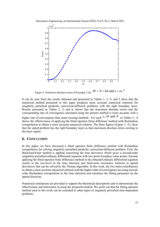
Figure 2: Pointwise absolute errors of Example 1 for
2
10
32 and
M N 
   
Example 2: Consider the following time-dependent convection-diffusion problem:
 
2 3
2 2 3
2
1 1
(1 sin( )) (1 sin( )) 1 (1 )sin( )
2 2 2
( , ) (0,1) (0,1]
( ,0) 0, 0 1
(0, ) (1, ) 0, 0 1
u u u t
x x x u x x t t t
t x x
x t
u x x
u t u t t
   
            
  
 
  
   
As the exact solution ( , )
u x t is unknown, we use the double mesh principle

12
Table 5: Comparison of maximum absolute errors obtained by present method for Example 2 at the
M N
 32/16 64/ 32 128/ 64 256/128
With fitting factor
0
10 3.8982e-05 1.0566e-05 2.7520e-06 7.0238e-07
1
10 3.1182e-04 8.6811e-05 2.2884e-05 5.8797e-06
2
10 1.6457e-03 6.4773e-04 1.9137e-04 5.0168e-05
3
10 1.7926e-03 9.8907e-04 5.1915e-04 2.5586e-04
4
10 1.7926e-03 9.8907e-04 5.1957e-04 2.6634e-04
0
10 4.0628e-05 1.0975e-05 2.8544e-06 7.2796e-07
1
10 5.1449e-04 1.3026e-04 3.2566e-05 8.1845e-06
2
10 3.6028e-02 1.5329e-02 4.5671e-03 9.9486e-04
3
10 1.1039e-01 9.7292e-02 7.4558e-02 4.6373e-02
4
10 1.2702e-01 1.2773e-01 1.2467e-01 1.1760e-01
Table 6: Comparisons of the corresponding order of convergence for Example 2 at /
M N
 32/16 64/ 32 128/ 64
With fitting factor
0
10 1.8834 1.9409 1.9702
1
10 1.8448 1.9235 1.9605
2
10 1.3452 1.7590 1.9315
3
10 0.8579 0.9299 1.0208
4
10 0.8579 0.9288 0.9640
0
10 1.8883 1.9430 1.9713
1
10 1.9817 2.0000 1.9924
2
10 1.2329 1.7469 2.1987
3
10 0.1822 0.3840 0.6851
4
10 -0.0080 0.0350 0.0842

13
Figure 3: Pointwise absolute errors of Example 2 for
4
10
64 and
M N 
   
It can be seen from the results obtained and presented in Tables 1, 3, 4, and 5 show that the
numerical method presented in this paper produces more accurate numerical solutions for
singularly perturbed parabolic convection-diffusion problems with the right boundary layer.
Results presented in Tables 2, 3, and 6, shows that the maximum absolute errors and the
corresponding rate of convergence calculated using the present method is more accurate with a
higher rate of convergence than some existing methods. For each , and
M N
 in Tables 2 - 6
shows the effectiveness of applying the fitted operator finite difference method with Richardson
extrapolation to obtain a more accurate numerical solution. The three figures (Figure 1 -3), show
that the stated problem has the right boundary layer so that maximum absolute errors existing in
the layer region.
6. CONCLUSION
In this paper, we have discussed a fitted operator finite difference method with Richardson
extrapolation for solving singularly perturbed parabolic convection-diffusion problem. First, the
Backward-Euler method is applied concerning the time derivative which gives a second-order
singularly perturbed ordinary differential equation with two-point boundary value points. Second,
applying the fitted operator finite difference method on the obtained ordinary differential equation
results in the two-level in the time direction and three-term recurrence relations in spatial
derivatives that can be solved by the Thomas algorithm. In this work, the two main contributions
to obtain a more accurate numerical solution with the higher order of convergence are using second-
order Richardson extrapolation in the time direction and introduce the fitting parameter on the
spatial direction.
Numerical simulations are provided to support the theoretical descriptions and to demonstrate the
effectiveness and betterment of using the proposed method. We point out that the fitting operator
method used in this work can be extended to other types of singularly perturbed time-dependent
problems.

14
REFERENCE
[1] J. B., Munyakazi, A Robust Finite Difference Method for Two-Parameter Parabolic Convection-
Diffusion Problems, An International Journal of Applied Mathematics & Information Sciences, Vol.
9(6), , (2015), 2877-2883.
[2] C. Clavero, J. C. Jorge, F. Lisbona, A uniformly convergent scheme on a non-uniform mesh for
convection-diffusion parabolic problems, Journal of Computational and Applied Mathematics 154(2)
(2003) 415-429.
[3] C. Yanping and L.B Liu, An adaptive grid method for singularly perturbed time-dependent convection-
diffusion problems, Commun. Comput. Phys. Vol. 20 (5), (2016), pp 1340-135.
[4] D. Pratibhamoy and M.Volker, Numerical solution of singularly perturbed convection-diffusion-
reaction problems with two small parameters, BIT Numer Math, (2015), DOI 10.1007/s10543-015-
0559-8.
[5] G.D. Smith, Numerical solution of partial differential equations, Finite difference methods, Third
Edition, Clarendon Press, Oxford, 1984.
[6] H.G. Roos, M. Stynes and L. Tobiska, Robust numerical methods for singularly perturbed differential
equations, Convection-diffusion-reaction and flow problems, Springer-Verlag Berlin Heidelberg,
Second Edition; 2008.
[7] J.J.H. Miller, E. O’Riordan and G.I., Shishkin, Fitted numerical methods for singular perturbation
problems, Error estimate in the maximum norm for linear problems in one and two dimensions, World
Scientific, 1996.
[8] K. Mukherjee, S. Natesan, Richardson extrapolation technique for singularly perturbed parabolic
convection-diffusion problems, Computing 92(1), (2011) 1-32.
[9] M. K. Kadalbajoo, A. Awasthi, A parameter uniform difference scheme for singularly perturbed
parabolic problem in one space dimension, Applied Mathematics and Computations 183(1) (2006) 42-
60.
[10] M. K. Ranjan, D. Vijay, K. Noopur, Spline in Compression Methods for Singularly Perturbed 1D
Parabolic Equations with Singular Coefficients, Open Journal of Discrete Mathematics, 2, (2012), 70-
77, http://dx.doi.org/10.4236/ojdm.2012.22013.
[11] R. Pratima and K. K. Sharma, Singularly perturbed parabolic differential equations with turning point
and retarded arguments, IAENG International Journal of Applied Mathematics, (2015), 45:4,
IJAM_45_4_20.
[12] S. Gowrisankar, S. Natesan, Robust numerical scheme for singularly perturbed convection-diffusion
parabolic initial–boundary-value problems on equidistributed grids, Computer Physics
Communications, 185, (2014), 2008-2019.
[13] S. Gowrisankar, S. Natesan, Robust numerical scheme for singularly perturbed convection-diffusion
parabolic initial-boundary-value problems on equidistributed grids, Computer Modelling in
Engineering & Sciences 88(4) (2012) 245-267.
[14] V. Kumar and B. Srinivasan, A novel adaptive mesh strategy for singularly perturbed parabolic
convection-diffusion problems, Differ Equ Dyn Syst, (2017), DOI 10.1007/s12591-017-0394-2.
[15] Y. Suayip and S. Niyazi, Numerical solutions of singularly perturbed one-dimensional parabolic
convection-diffusion problems by the Bessel collocation method, Applied Mathematics and
Computation 220, (2013), 305–315.
[16] T. A. Bullo, G. F. Duressa and G. A. Degla, Robust Finite Difference Method for Singularly Perturbed
Two-Parameter Parabolic Convection-Diffusion Problems, International Journal of Computational
Methods, Vol. 18, No. 2 (2021) 2050034.

FITTED OPERATOR FINITE DIFFERENCE METHOD FOR SINGULARLY PERTURBED PARABOLIC CONVECTION-DIFFUSION TYPE

Recommended

Recommended

More Related Content

What's hot

What's hot (20)

Similar to FITTED OPERATOR FINITE DIFFERENCE METHOD FOR SINGULARLY PERTURBED PARABOLIC CONVECTION-DIFFUSION TYPE

Similar to FITTED OPERATOR FINITE DIFFERENCE METHOD FOR SINGULARLY PERTURBED PARABOLIC CONVECTION-DIFFUSION TYPE (20)

More from ieijjournal

More from ieijjournal (20)

Recently uploaded

Recently uploaded (20)

FITTED OPERATOR FINITE DIFFERENCE METHOD FOR SINGULARLY PERTURBED PARABOLIC CONVECTION-DIFFUSION TYPE