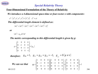
Downloaded 1,044 times
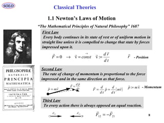


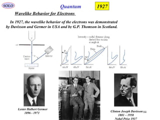
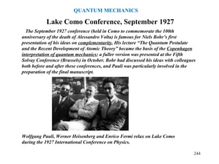
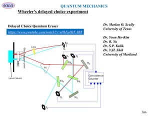
![22
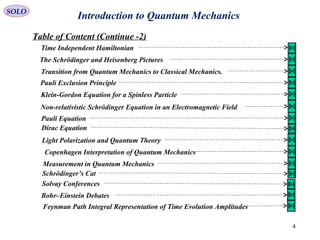
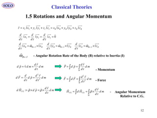
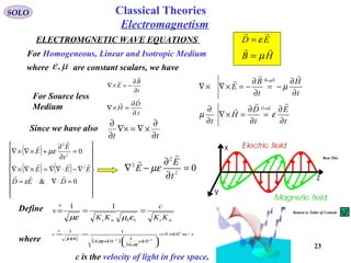
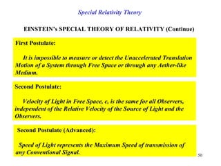
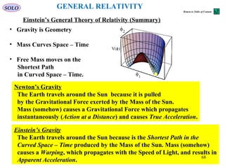
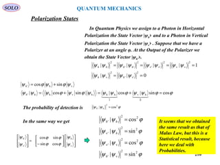
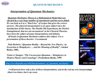
MAXWELL’s EQUATIONS
SOLO
Magnetic Field IntensityH
[ ]1−
⋅mA
Electric DisplacementD
[ ]2−
⋅⋅ msA
Electric Field IntensityE
[ ]1−
⋅mV
Magnetic InductionB
[ ]2−
⋅⋅ msV
Electric Current DensityeJ
[ ]2−
⋅mA
Free Electric Charge Distributioneρ [ ]3−
⋅⋅ msA
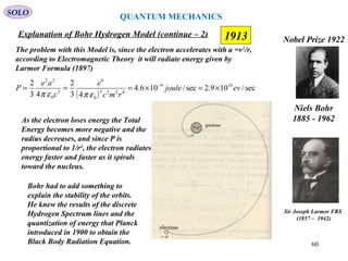
1. AMPÈRE’S CIRCUIT LAW (A) 1821 eJ
t
D
H
+
∂
∂
=×∇
2. FARADAY’S INDUCTION LAW (F) 1831
t
B
E
∂
∂
−=×∇
3. GAUSS’ LAW – ELECTRIC (GE) ~ 1830
eD ρ=⋅∇
4. GAUSS’ LAW – MAGNETIC (GM) 0=⋅∇ B
André-Marie Ampère
1775-1836
Michael Faraday
1791-1867
Karl Friederich Gauss
1777-1855
James Clerk Maxwell
(1831-1879)
1865
Electromagnetism
MAXWELL UNIFIED ELECTRICITY AND MAGNETISM
Classical Theories](https://image.slidesharecdn.com/5-introductiontoquantummechanics-sololaptop-150813162751-lva1-app6891/85/5-introduction-to-quantum-mechanics-22-320.jpg)

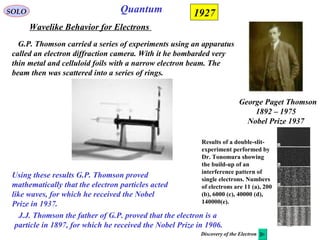
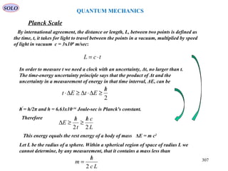
![40
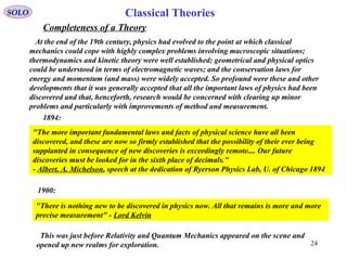
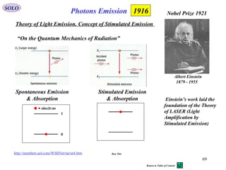
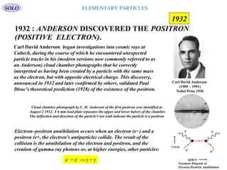
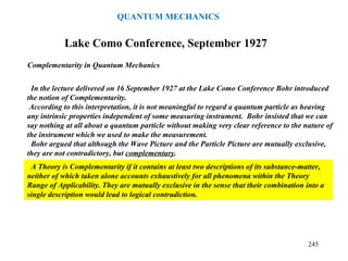
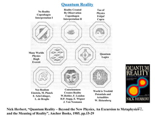
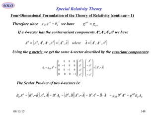
Physical Laws of RadiometrySOLO
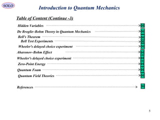
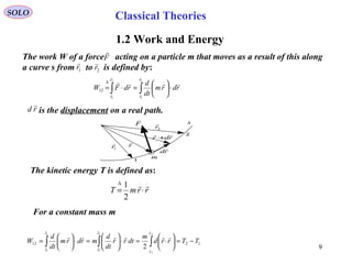
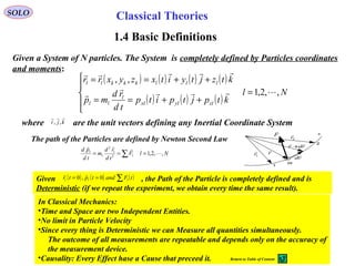
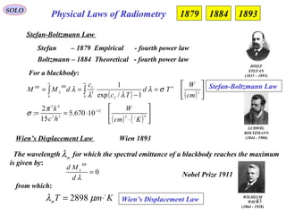
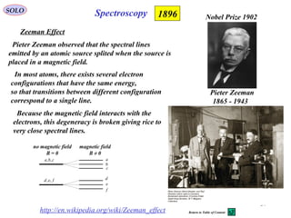
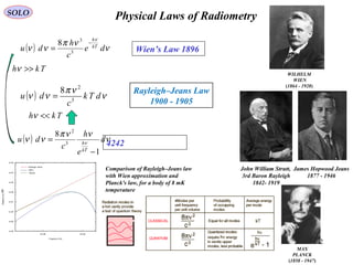
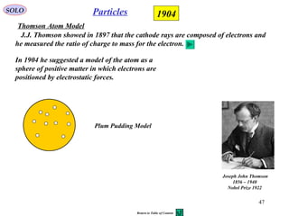
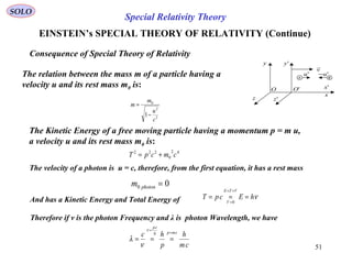
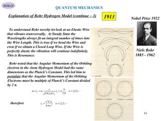
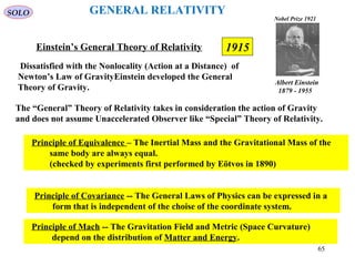
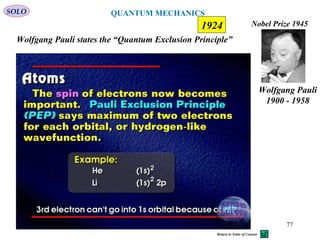
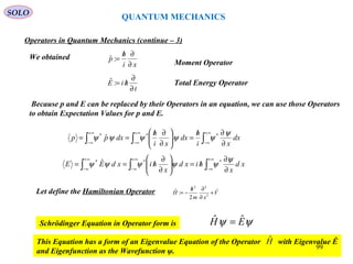
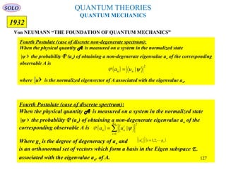
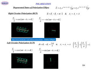
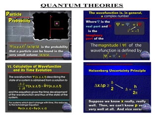
Rayleigh–Jeans Law
Comparison of Rayleigh–Jeans law with
Wien approximation and Planck's law, for
a body of 8 mK temperature
In 1900, the British physicist Lord Rayleigh derived
the λ−4
dependence of the Rayleigh–Jeans law based on
classical physical arguments.[3]
A more complete
derivation, which included the proportionality constant,
was presented by Rayleigh and Sir James Jeans in
1905. The Rayleigh–Jeans law revealed an important
error in physics theory of the time. The law predicted
an energy output that diverges towards infinity as
wavelength approaches zero (as frequency tends to
infinity) and measurements of energy output at short
wavelengths disagreed with this prediction.
John William Strutt,
3rd Baron Rayleigh
1842- 1919
James Hopwood Jeans
1877 - 1946
Rayleigh considered the radiation inside a cubic
cavity of length L and temperature T whose walls
are perfect reflectors as a series of standing
electromagnetic waves. At the walls of the cube, the
parallel component of the electric field and the
orthogonal component of the magnetic field must
vanish. Analogous to the wave function of a
particle in a box, one finds that the fields are
superpositions of periodic functions. The three
wavelengths λ1, λ2 and λ3, in the three directions
orthogonal to the walls can be: ,2,1,,
2
=== i
i
i
nzyxi
n
Lλ
1900 1905](https://image.slidesharecdn.com/5-introductiontoquantummechanics-sololaptop-150813162751-lva1-app6891/85/5-introduction-to-quantum-mechanics-40-320.jpg)

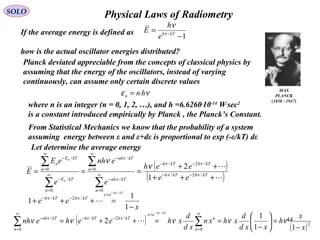
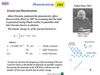
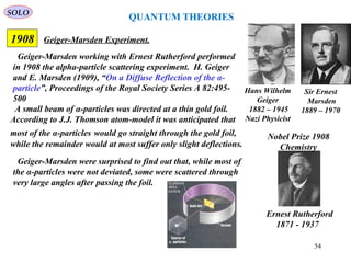


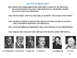
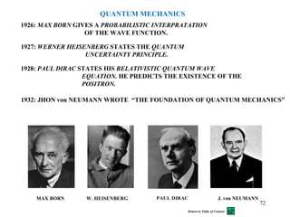
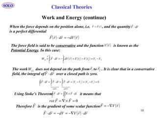
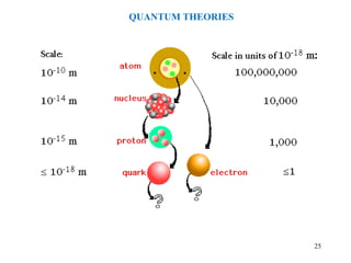
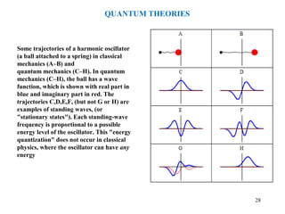
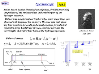
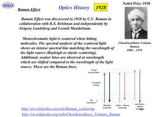
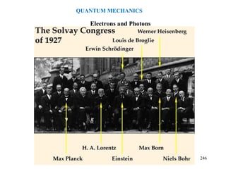
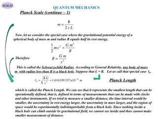
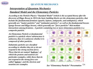
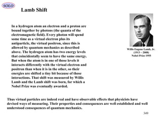
![QUANTUM THEORIES
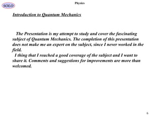
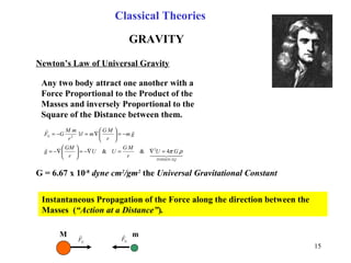
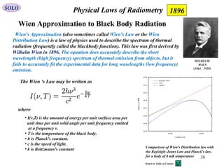
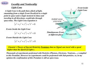
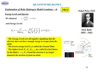
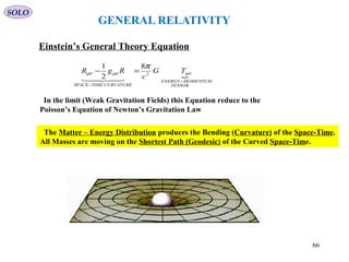
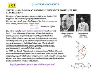
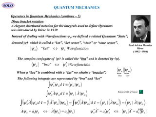
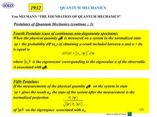
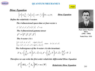
Werner Heisenberg, Max Born, and Pascal Jordan formulate Quantum
Matrix Mechanics.
QUANTUM MATRIX MECHANICS.
Werner Karl Heisenberg
(1901 – 1976)
Nobel Price 1932
Max Born
(1882–1970)
Nobel Price 1954
Ernst Pascual Jordan
(1902 – 1980)
Nazi Physicist
http://en.wikipedia.org/wiki/Matrix_mechanics
1925
Matrix mechanics was the first conceptually autonomous and
logically consistent formulation of quantum mechanics. It extended the
Bohr Model by describing how the quantum jumps occur. It did so by
interpreting the physical properties of particles as matrices that evolve
in time. It is equivalent to the Schrödinger wave formulation of
quantum mechanics, and is the basis of Dirac's bra-ket notation for the
wave function.
SOLO
In 1928, Einstein nominated Heisenberg, Born, and Jordan for the
Nobel Prize in Physics, but Heisenberg alone won the 1932 Prize "for
the creation of quantum mechanics, the application of which has led to
the discovery of the allotropic forms of hydrogen",[47]
while
Schrödinger and Dirac shared the 1933 Prize "for the discovery of new
productive forms of atomic theory".[47]
On 25 November 1933, Born
received a letter from Heisenberg in which he said he had been delayed
in writing due to a "bad conscience" that he alone had received the
Prize "for work done in Gottingen in collaboration — you, Jordan and
I."[48]
Heisenberg went on to say that Born and Jordan's contribution
to quantum mechanics cannot be changed by "a wrong decision from
the outside." 78
Return to Table of Content](https://image.slidesharecdn.com/5-introductiontoquantummechanics-sololaptop-150813162751-lva1-app6891/85/5-introduction-to-quantum-mechanics-78-320.jpg)
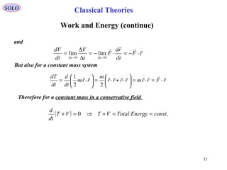
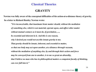
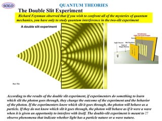
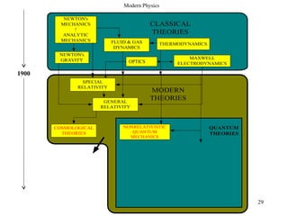
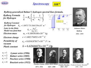
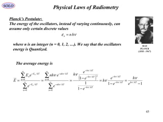
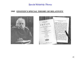
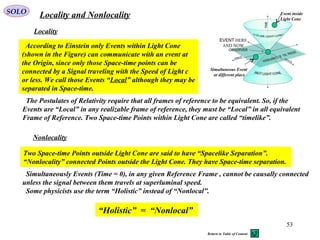
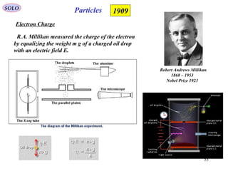
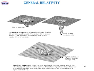
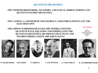
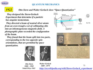
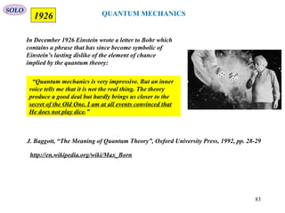
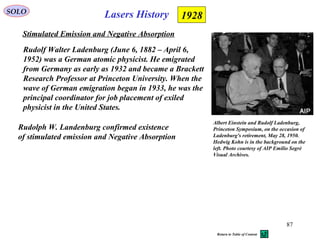
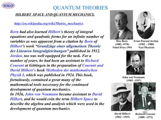
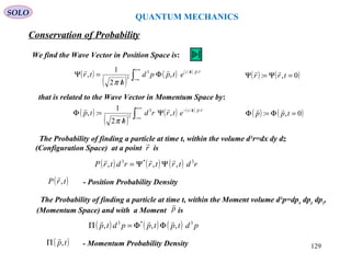
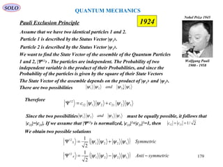
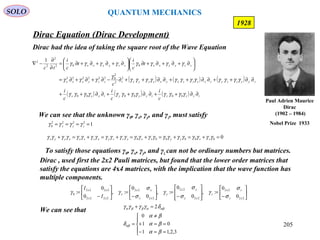
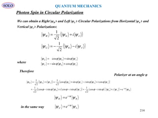
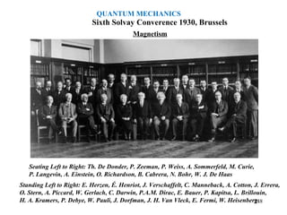
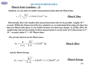
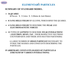
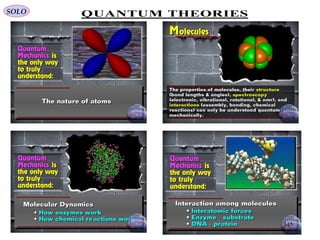
![Spin
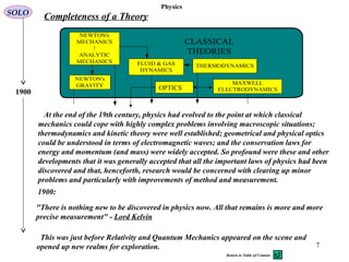
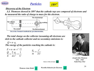
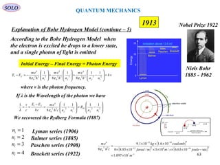
In quantum mechanics and particle physics, Spin is an intrinsic form of angular
momentum carried by elementary particles, composite particles (hadrons), and
atomic nuclei. Spin is a solely quantum-mechanical phenomenon; it does not have a
counterpart in classical mechanics (despite the term spin being reminiscent of
classical phenomena such as a planet spinning on its axis).[
Spin is one of two types of angular momentum in quantum mechanics, the other
being orbital angular momentum. Orbital angular momentum is the quantum-
mechanical counterpart to the classical notion of angular momentum: it arises
when a particle executes a rotating or twisting trajectory (such as when an electron
orbits a nucleus).The existence of spin angular momentum is inferred from
experiments, such as the Stern–Gerlach experiment, in which particles are observed
to possess angular momentum that cannot be accounted for by orbital angular
momentum alone.[
http://en.wikipedia.org/wiki/Spin_(physics)
In some ways, spin is like a vector quantity; it has a definite “magnitude”; and it has
a "direction" (but quantization makes this "direction" different from the direction
of an ordinary vector). All elementary particles of a given kind have the same
magnitude of spin angular momentum, which is indicated by assigning the particle a
spin quantum number.[2]
However, in a technical sense, spins are not strictly vectors,
and they are instead described as a related quantity: a Spinor. In particular, unlike a
Euclidean vector, a spin when rotated by 360 degrees can have its sign reversed
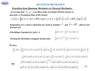
QUANTUM MECHANICS
80](https://image.slidesharecdn.com/5-introductiontoquantummechanics-sololaptop-150813162751-lva1-app6891/85/5-introduction-to-quantum-mechanics-80-320.jpg)
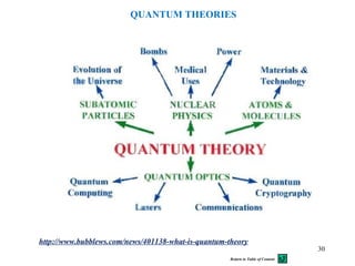
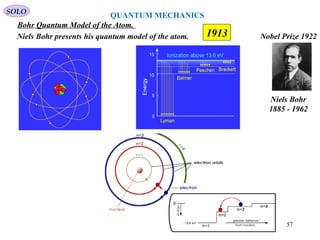
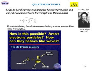
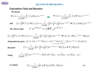
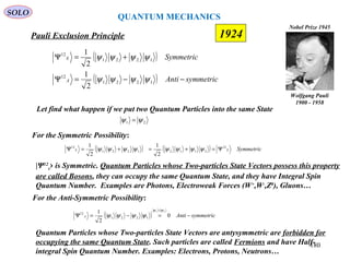
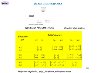
![ERWIN SCHRÖDINGER STAES THE NONRELATIVISTIC
QUANTUM WAVE EQUATION AND FORMULATES THE
QUANTUM MECHANICS. HE PROVES THAT WAVE AND
MATRIX FORMULATIONS ARE EQUIVALENT
1926
In January 1926, Schrödinger published in Annalen der Physik the paper
"Quantisierung als Eigenwertproblem" [“Quantization as an Eigenvalue Problem”]
on wave mechanics and presented what is now known as the Schrödinger equation. In
this paper, he gave a "derivation" of the wave equation for time-independent systems
and showed that it gave the correct energy eigenvalues for a hydrogen-like atom. This
paper has been universally celebrated as one of the most important achievements of the
twentieth century and created a revolution in quantum mechanics and indeed of all
physics and chemistry. A second paper was submitted just four weeks later that solved
the quantum harmonic oscillator, rigid rotor, and diatomic molecule problems and
gave a new derivation of the Schrödinger equation. A third paper in May showed the
equivalence of his approach to that of Heisenberg.
http://en.wikipedia.org/wiki/Erwin_Schr%C3%B6dinger
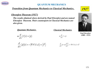
QUANTUM MECHANICS
Erwin Rudolf Josef
Alexander Schrödinger
(1887 – 1961)
Nobel Prize 1933
SOLO
81](https://image.slidesharecdn.com/5-introductiontoquantummechanics-sololaptop-150813162751-lva1-app6891/85/5-introduction-to-quantum-mechanics-81-320.jpg)
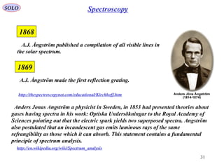
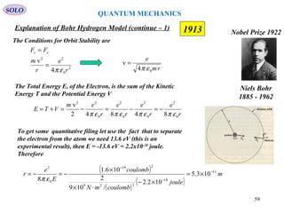
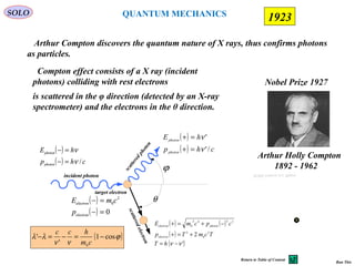
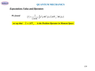
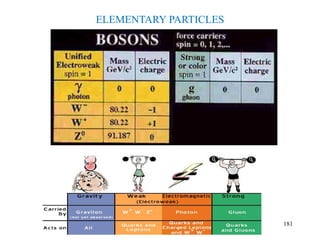
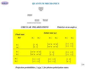
![MAX BORN GIVES A PROBABILISTIC INTERPRATATION
OF THE WAVE FUNCTION.
1926
Max Born
(1882–1970)
Nobel Price 1954
Max Born wrote in 1926 a short paper on collisions between particles,
about the same time as Schrödinger paper “Quantization as an
Eigenvalue Problem”. Born rejected the Schrödinger Wave Field
approach. He had been influenced by a suggestion made by Einstein
that, for photons, the Wave Field acts as strange kind of ‘phantom’ Field
‘guiding’ the photon particles on paths which could therefore be
determined by Wave Interference Effects.
Max Born reasoned that the Square of the Amplitude of the Waveform in some specific region
of configuration space is related to the Probability of finding the associated quantum particle in
that region of configuration space.
Since Probability is a real number, and the integral of all Probabilities over all regions of
configuration space, the Wave Function must satisfy
1*
=∫
+∞
∞−
dVψψ Condition of Normalization of the Wave Function
Therefore the probability of finding the particle
between a and b is given by
[ ] ( ) ( )∫=≤≤
b
a
xdxxbXaP ψψ *
Einstein rejected this interpretation. In a 1926 letter to Max Born, Einstein
wrote: "I, at any rate, am convinced that He [God] does not throw dice."[
QUANTUM MECHANICS
SOLO
82
Return to Table of Content](https://image.slidesharecdn.com/5-introductiontoquantummechanics-sololaptop-150813162751-lva1-app6891/85/5-introduction-to-quantum-mechanics-82-320.jpg)
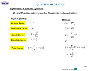
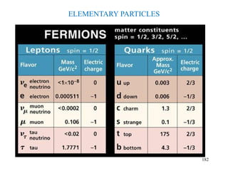
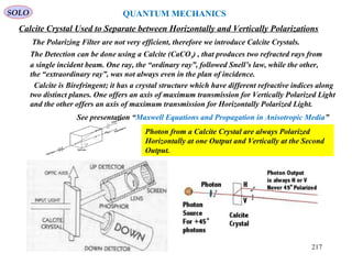
![ERWIN SCHRÖDINGER STAES THE NONRELATIVISTIC
QUANTUM WAVE EQUATION AND FORMULATES THE
QUANTUM MECHANICS. HE PROVES THAT WAVE AND
MATRIX FORMULATIONS ARE EQUIVALENT
1926
Following Max Planck's quantization of light (see black body radiation),
Albert Einstein interpreted Planck's quanta to be photons, particles of light,
and proposed that the energy of a photon is proportional to its frequency, one
of the first signs of wave–particle duality. Since energy and momentum are
related in the same way as frequency and wavenumber in special relativity, it
followed that the momentum p of a photon is proportional to its wavenumber k.
c
k
h
hwherekh
h
p
c πν
λ
π
πλ
νλ 22
:,
2
:
/=
===//==
Louis de Broglie hypothesized that this is true for all particles, even particles such as electrons. He
showed that, assuming that the matter waves propagate along with their particle counterparts,
electrons form standing waves, meaning that only certain discrete rotational frequencies about the
nucleus of an atom are allowed.[7]
These quantized orbits correspond to discrete energy levels, and
de Broglie reproduced the Bohr model formula for the energy levels. The Bohr model was based on
the assumed quantization of angular momentum:
hn
h
nL /==
π2
According to de Broglie the electron is described by a wave and a whole number of wavelengths
must fit along the circumference of the electron's orbit: n λ = 2 π r
http://en.wikipedia.org/wiki/Schr%C3%B6dinger_equation
Historical Background and Development
QUANTUM MECHANICS
Erwin Rudolf Josef
Alexander Schrödinger
(1887 – 1961)
Nobel Prize 1933
SOLO
91](https://image.slidesharecdn.com/5-introductiontoquantummechanics-sololaptop-150813162751-lva1-app6891/85/5-introduction-to-quantum-mechanics-91-320.jpg)

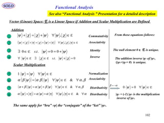
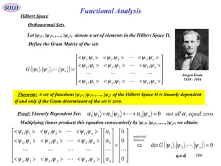
![105
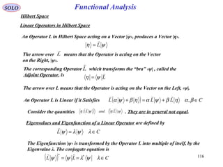
Functional AnalysisSOLO
Inner Product Using Dirac Notation
If E is a complex Linear Space, for the Inner Product (bracket) < | >
between the elements (a complex number) is defined by:
E∈∀ 321 ,, ψψψ
*
1221 || >>=<< ψψψψ1 Commutative Law
Using to we can show that:1 4
If E is an Inner Product Space, than we can induce the Norm: [ ] 2/1
111 , ><= ψψψ
2 Distributive Law><+>>=<+< 3121321 ||| ψψψψψψψ
3 C∈><>=< αψψαψψα 2121 ||
4
00|&0| 11111 =⇔>=<≥>< ψψψψψ
( ) ( ) ( )
><+><=><+><=>+<=>+< 1312
1
*
31
*
21
2
*
321
1
132 |||||| ψψψψψψψψψψψψψψ
( ) ( ) ( )
><=><=><=>< 21
*
1
*
12
*
3
*
12
1
21 |||| ψψαψψαψψαψαψ
( ) ( )
*
1
1
111
2
11 |000|0|0|00|0| ><=>=<⇒><+><=>+>=<< ψψψψψψ](https://image.slidesharecdn.com/5-introductiontoquantummechanics-sololaptop-150813162751-lva1-app6891/85/5-introduction-to-quantum-mechanics-105-320.jpg)
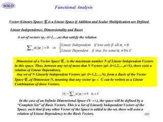
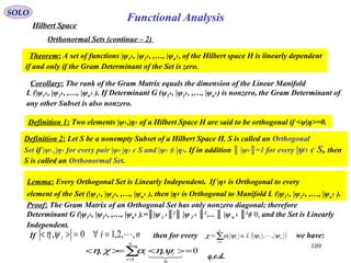
![107
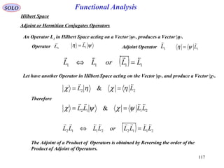
Functional Analysis
SOLO
Hilbert Space
A Complete Space E is a Metric Space (in our case ) in which every
Cauchy Sequence converge to a limit inside E.
( ) 2121, ψψψψρ −=
David Hilbert
1862 - 1943
A Linear Space E is called a Hilbert Space if E is an Inner Product Space that is
complete with respect to the Norm induced by the Inner Product ||ψ1||=[< ψ1, ψ1>]1/2
.
Equivalently, a Hilbert Space is a Banach Space (Complete Metric Space) whose
Norm is induced by the Inner Product ||ψ1||=[< ψ1, ψ1>]1/2
.
Orthogonal Vectors in a Hilbert Space:
Two Vectors |η› and |ψ› are Orthogonal if 0|| == ηψψη
Theorem: Given a Set of Linearly Independent Vectors in a Hilbert
Space |ψi› (i=1,…,n) and any Vector |ψm› Orthogonal to all |ψi›,
than it is also Linearly Independent.
Proof: Suppose that the Vector |ψm› is Linearly Dependent on |ψi› (i=1,…,n)
∑=
=≠
n
i iim 1
0 ψαψ
But ∑=
==≠
n
i imimm 1
0
00
ψψαψψ
We obtain a inconsistency, therefore |ψm› is Linearly Independent on |ψi› (i=1,…,n)
Therefore in a Hilbert Space, of Finite or Infinite Dimension, by finding the Maximum
Set of Orthogonal Vectors we find a Basis that “Complete” covers the Space.
q.e.d.](https://image.slidesharecdn.com/5-introductiontoquantummechanics-sololaptop-150813162751-lva1-app6891/85/5-introduction-to-quantum-mechanics-107-320.jpg)
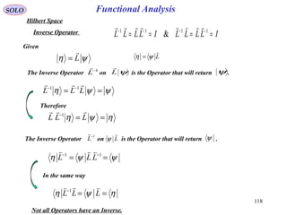


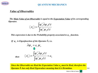
![QUANTUM MECHANICS
SOLO
The condition that the probability of finding the particle somewhere to be unity, we deduce that
should be normalized to unity.( )tr,
Ψ
( ) ( )
( )
( ) ( ) ( )[ ]
( ) ( ) ( )[ ]
( )
( ) ( ) ( ) ( ) ( )[ ] ( )( )
∫ ∫∫
∫ ∫∫∫
∞+
∞−
∞+
∞−
⋅−//
∞+
∞−
−//−
+∞
∞−
+∞
∞−
⋅−//−
+∞
∞−
⋅−//
ΦΦ
/
=
ΦΦ
/
=ΨΨ=
rpphitpEpEhi
rptpEhirptpEhi
erdetptppdpd
h
etppdetppdrd
h
trtrrd
'/3'/*33
3
/3''/*33
3
*3
,,''
2
1
,,''
2
1
,,1
π
π
Use
( )
( )( ) ( )( ) ( )( ) ( )( )
( ) ( ) ( ) ( )''''
2
1
2
1
2
1
2
1 '/'/'/'/3
3
ppppppppezd
h
eyd
h
exd
h
erd
h
zzyyxx
zpphiypphixpphirpphi zzyyxx
−=−−−=
/
/
/
=
/ ∫∫∫∫
∞+
∞−
−//
∞+
∞−
−//∞+
∞−
−//
∞+
∞−
⋅−//
δδδδ
ππππ
( ) ( ) ( ) ( ) ( ) ( ) ( )[ ]
( )∫ ∫∫
+∞
∞−
+∞
∞−
−//−
−ΦΦ=ΨΨ ',,'',, '/*33*3
ppetptppdpdtrtrrd tpEpEhi
δ
Finally we obtain
( ) ( ) ( ) ( ) 1,,',, *3*3
=ΦΦ=ΨΨ ∫∫
+∞
∞−
tptppdtrtrrd
Return to Conservation
of Probability
Conservation of Probability
130](https://image.slidesharecdn.com/5-introductiontoquantummechanics-sololaptop-150813162751-lva1-app6891/85/5-introduction-to-quantum-mechanics-130-320.jpg)
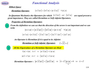
![QUANTUM MECHANICS
Conservation of Probability
SOLO
Since at any time t, the Probability of finding the particle somewhere is unity, and the
Probability of the particle being in the Momentum Space is unity we have
( ) ( ) ( ) 1,,, 3*3
=ΨΨ= ∫∫ rdtrtrrdtrP
( ) ( ) ( ) 1,,, 3*3
=ΦΦ=Π ∫∫ pdtptppdtp
( ) ( ) ( ) ( ) ( ) 0,,,,, 3**3
=
Ψ
∂
∂
Ψ+ΨΨ
∂
∂
=
∂
∂
∫∫ rdtr
t
trtrtr
t
rdtrP
t
Use Schrödinger equation : ( ) ( ) ctrV
m
h
tr
t
hi <<Ψ
−∇
/
=Ψ
∂
∂
/− v,
2
, 2
2
( ) ( ) ctrV
m
h
tr
t
hi
VV
<<Ψ
−∇
/
=Ψ
∂
∂
/
=
v,
2
, *2
2
*
*
and its conjugate:
Let consider a finite Region T in the Position Space:
Since: ( ) ( ) ( )( ) ( )( ) ( ) ( )trVtrtrtrVtrtrV ,,,,,, ****
ΨΨ=ΨΨ=ΨΨ
( ) ( ) ( ) ( ) ( ) rdtrV
m
h
trtrtrV
m
h
hi
rdtrP
t
32
2
**2
2
3
,
2
,,,
2
1
, ∫∫ ΤΤ
Ψ
−∇
/
Ψ−ΨΨ
−∇
/
/
=
∂
∂
( ) ( ) ( ) ( ) ( )[ ]
( ) ( ) ( ) ( )[ ]∫
∫∫
Ψ∇Ψ−ΨΨ∇⋅∇
/
=
Ψ∇Ψ−ΨΨ∇
/
=
∂
∂
T
TT
rdtrtrtrtr
im
h
rdtrtrtrtr
im
h
rdtrP
t
3**
32**23
,,,,
2
,,,,
2
,
131](https://image.slidesharecdn.com/5-introductiontoquantummechanics-sololaptop-150813162751-lva1-app6891/85/5-introduction-to-quantum-mechanics-131-320.jpg)
![QUANTUM MECHANICS
Conservation of Probability
SOLO
( ) ( ) ( ) ( ) ( )[ ] ∫∫∫ ⋅∇−=ΨΨ∇−Ψ∇Ψ⋅∇
/
−=
∂
∂
TTT
rdjrdtrtrtrtr
im
h
rdtrP
t
33**3
,,,,
2
,
where
( ) ( ) ( ) ( )[ ]
( ) ( )[ ]trtr
m
h
trtrtrtr
im
h
j
,,Im
,,,,
2
:
*
**
Ψ∇Ψ
/
=
ΨΨ∇−Ψ∇Ψ
/
=
Since in the Equation above we have any time independent Spatial Volume T we can write
( ) ( ) 0,, =⋅∇+
∂
∂
trjtrP
t
Therefore is the Probability Current Density.( )trj ,
132
( ) ( ) ( ) rdtrtrrdtrP 3*3
,,,
ΨΨ= ( )trP ,
- Position Probability Density](https://image.slidesharecdn.com/5-introductiontoquantummechanics-sololaptop-150813162751-lva1-app6891/85/5-introduction-to-quantum-mechanics-132-320.jpg)
![QUANTUM MECHANICS
Conservation of Probability
SOLO
The Probability Current Density is( )trj ,
133
Return to Table of Content
Connection with classical mechanics
The wave function can also be written in the complex exponential (polar) form
( ) ( ) ( )
( ) ( ) R∈=Ψ /
trStrRetrRtr htrSi
,,,,, /,
The Probability is defined as ( ) ( ) ( ) ( )trRtrtrtrP ,,,:, 2*
=ΨΨ=
( ) ( ) ( )[ ]
∇
/
−∇−
∇
/
+∇
/
=
∇
/
−∇−
∇
/
+∇
/
=
∇−∇
/
=Ψ∇Ψ−Ψ∇Ψ
/
=
/−/−////−
/−///−
SR
h
i
RRSR
h
i
RR
im
h
SeR
h
i
ReeRSeR
h
i
ReeR
im
h
eReReReR
im
h
im
h
j
hSihSihSihSihSihSi
hSihSihSihSi
2
2
22
:
//////
////**
Therefore
m
S
j
∇
= ρ:
Define
m
Sj ∇
==
ρ
:v Probability Current Velocity
( ) ( ) ( )( ) 0,v,, =⋅∇+
∂
∂
trtrtrP
t
ρWe have Conservation of Probability](https://image.slidesharecdn.com/5-introductiontoquantummechanics-sololaptop-150813162751-lva1-app6891/85/5-introduction-to-quantum-mechanics-133-320.jpg)
![[ ] ABBABA −=:,
Commutator of two Operators A and B
[ ] [ ]ABBA ,, −=
[ ] [ ] [ ]CABACBA ,,, +=+
[ ] [ ] [ ]CABCBACBA ,,, +=
[ ][ ] [ ][ ] [ ][ ] 0,,,,,, =++ BACACBCBA
General Commutator Properties
If A B = B A we say that the two Operators A and B Commute, and then [A,B] = 0 .
In general A B ≠ B A and we say that A and B don’t commute.
Theorem: A and B Commute if and only if they have the same Eigenfunctions ψi
nibBaA iiiiii ,,1& === ψψψψ
Using Expansion Theorem any Vector
[ ] ( ) ( ) 0||,
0
11
=−Ψ=−Ψ=Ψ−Ψ=Ψ ∑∑ == iiiiii
n
i i
n
i iii abbaABBAABBABA ψψψψψψ
∑=
Ψ=Ψ
n
i ii1
ψψ
Proof: If A and B have the same Eigenfunctions ψi then
Therefore A and B Commute.
QUANTUM MECHANICS
Antisymmetry
Associativity
Jacobi Identity
SOLO
150](https://image.slidesharecdn.com/5-introductiontoquantummechanics-sololaptop-150813162751-lva1-app6891/85/5-introduction-to-quantum-mechanics-150-320.jpg)
![[ ] ABBABA −=:,
Commutator of two Operators A and B
Theorem: A and B Commute if and only if they have the same Eigenfunctions ψn
iii aA ψψ =Suppose that A have a complete set of Eigenfunctions
Proof (continue - 1): If A and B Commute, then they have the same Eigenfunctions ψn
then ( ) ( )ii
aA
i
ABBA
i BaABBA
iii
ψψψ
ψψ ==
==
Therefore Bψi and ψi are both Eigenfunctions of A, having the Eigenvalue ai, but this is
possible only if they differ by a constant which will call bi
iii bB ψψ =
Assume first that A has non-degenerate Eigenvalues ai
Therefore A and B have the same Eigenfunctions ψi , if ai are non-degenerate Eigenvalues. .
Now assume that A has a degenerate Eigenvalue ai, of degree α, with corresponding linearly
independent Eigenfunctions ψir (r=1,2,…,α). Since A B Commute (B ψi) is an Eigenfunction
of A belonging to the degenerated Eigenvalue ai. It follows that (B ψi) can be expanded in terms
of the linearly independent functions ψi1 , ψi2 ,…, ψiα
∑ =
=
α
ψψ 1s isisir cB
QUANTUM MECHANICS
SOLO
151](https://image.slidesharecdn.com/5-introductiontoquantummechanics-sololaptop-150813162751-lva1-app6891/85/5-introduction-to-quantum-mechanics-151-320.jpg)
![[ ] ABBABA −=:,
Commutator of two Operators A and B
Theorem: A and B Commute if and only if they have the same Eigenfunctions ψi
Proof (continue - 2): If A and B Commute, then they have the same Eigenfunctions ψi
Therefore A and B have the same Eigenfunctions , even if ai are degenerate Eigenvalues. .
{ } nsrrss isrsir ccB ,,1,1 ==∑=
α
ψψ
Let form a linear combination of the functions ψir with α constants dr (r=1,2,…,α) to be
defined ∑ ∑∑ = ==
=
α αα
ψψ 1 11 r s isrsrr irr cddB
If we can find constants biβ (β=1,..,α) such that αβ
α
,,2,11
==∑ =
sdbcd sis rsr
Then and is an
Eigenfunction of B and by its structure, is also an Eigenfunction of A. To find α
Eigenfunctions and Eigenvalues we must solve
( ) ∑∑ ∑∑ == ==
==
α
β
α αα
ψψψ 11 11 s issis isr rsrr irr dbcddB ∑ =
α
ψ1r irrd
{ }( ) 0,,2,1
1
1
=
−⇒==∑ =
α
α
α
α
d
d
Ibcsdbcd iissis isr
We find α Eigenvectors (d1,…,dα)T
and Eigenvalues biβ of Matrix {cis}.
Now assume that A has a degenerate Eigenvalue ai, of degree α, , then
since AB Commute, (Bψir)is an Eigenfunction of A, and
( )αψψ ,,1 == raA iriir
QUANTUM MECHANICS
SOLO
152](https://image.slidesharecdn.com/5-introductiontoquantummechanics-sololaptop-150813162751-lva1-app6891/85/5-introduction-to-quantum-mechanics-152-320.jpg)
![[ ] ABBABA −=:,
Commutator of two Operators A and B
Examples
xhipBxA x ∂∂/−=== /&
[ ] ( ) ( ) ψψ
ψ
ψψ hix
xx
xhixppxpx xxx /=
∂
∂
−
∂
∂
/−=−=,
In the same way [ ] [ ] ψψψψ hipzhipy zy /=/= ,&,
[ ] [ ] [ ] hipzhipyhipx zyx /=/=/= ,&,&,
1
3
t
hiEBtA
∂
∂
/=== &
[ ] ( ) ψψ
ψ
ψψ hit
tt
thitp
t
hitEt x /−=
∂
∂
−
∂
∂
/=
−
∂
∂
/=,
Since this is true for all State Vectors ψ
[ ] hiEt /−=,
QUANTUM MECHANICS
SOLO
[ ] ( )[ ] ( ) ψψψψψ hirhirrhipr
I
/=∇/=∇−∇/−=
, [ ] hipr /=
,
∇/−=== hipBrA
&2
[ ] [ ] [ ] [ ] [ ] [ ] 0,,&0,,&0,, ====== yxzxzy pzpzpypypxpxalso
153
Return to Table of Content](https://image.slidesharecdn.com/5-introductiontoquantummechanics-sololaptop-150813162751-lva1-app6891/85/5-introduction-to-quantum-mechanics-153-320.jpg)
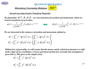
![ΨΨ=ΨΨ= ||&|| BBAA
Heisenberg Uncertainty Relations
Consider two Observable A and B, and a given Normalized State |Ψ›.
We define the Uncertainties ∆A and ∆B (Observable Variances) as
1| =ΨΨ
( )[ ] ( )[ ] 2/122/12
:&: BBBAAA −=∆−=∆
( ) ( ) 222222
2 AAAAAAAAA −=+−=−=∆ ( ) 222
BBB −=∆
Define
0
~
&0
~
:
~
&:
~
==
−=−=
BA
BBBAAA
[ ] [ ] [ ] [ ] [ ] [ ] [ ] [ ]
000
,,,,,,,
~
,
~
BABABABABBABBABBAABA +−−=−−−=−−=
Define the Linear but no Hermitian Operator
BiAC
constBiAC
~~
:
~~
:
*
*
λ
λλλ
−=
==+=
Werner Karl Heisenberg
(1901 – 1976)
Nobel Price 1932
1927
The Expectations (Observables Main Values) of A and B are given by:
QUANTUM MECHANICS
SOLO
154](https://image.slidesharecdn.com/5-introductiontoquantummechanics-sololaptop-150813162751-lva1-app6891/85/5-introduction-to-quantum-mechanics-154-320.jpg)
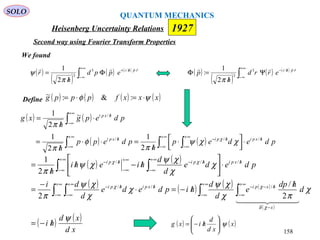
![Heisenberg Uncertainty Relations (continue – 1)
Define the Real and Nonnegative Function of λ
0||| ****
≥ΨΨ=ΨΨ=
Real
CCCCCC
( )( ) ( ) [ ]BAiBAABBAiBABiABiACC
~
,
~~~~~~~~~~~~~ 222222*
λλλλλλ −+=−−+=−+=
( ) [ ] [ ]
( ) ( ) [ ] 0,
~
,
~~~~
,
~~~
222
222222
≥−∆+∆=
−+=−+=
BAiBA
BAiBABAiBAf
λλ
λλλλλ
Since f (λ) is Real → i λ ‹[A,B]› is Real → ‹[A,B]› is Purely Imaginary → ‹[A,B]› 2
≤0
f (λ) has a nonnegative minimum for
[ ]
( )20
,
2 B
BAi
∆
=λ
( ) ( ) ( )
[ ]
( )
0
,
4
1
min 2
2
2
0 ≥
∆
+∆==
B
BA
Aff λλ ( ) ( ) [ ] 0,
4
1 222
≥−≥∆∆ BABA
QUANTUM MECHANICS
SOLO
155](https://image.slidesharecdn.com/5-introductiontoquantummechanics-sololaptop-150813162751-lva1-app6891/85/5-introduction-to-quantum-mechanics-155-320.jpg)
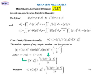
![Heisenberg Uncertainty Relations (continue – 2)
Since ∆A and ∆B are real and positive, we found
[ ]BABA ,
2
1
≥∆⋅∆
and
Therefore
2
&
2
&
2
h
pz
h
py
h
px zyx
/
≥∆⋅∆
/
≥∆⋅∆
/
≥∆⋅∆
2
h
Et
/
≥∆⋅∆
Heisenberg Uncertainty
Relation for Simultaneous
Position & Momentum
Measurements
Heisenberg Uncertainty
Relation for Simultaneous
Time & Energy
Measurements
1 [ ] [ ] [ ] hipzhipyhipx zyx /=/=/= ,&,&,
2 [ ] hiEt /−=,
QUANTUM MECHANICS
SOLO
156](https://image.slidesharecdn.com/5-introductiontoquantummechanics-sololaptop-150813162751-lva1-app6891/85/5-introduction-to-quantum-mechanics-156-320.jpg)


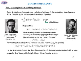
![QUANTUM MECHANICS
The Schrödinger and Heisenberg Pictures (continue – 2)
Werner Karl Heisenberg
(1901 – 1976)
Nobel Price 1932
Erwin Rudolf Josef
Alexander Schrödinger
(1887 – 1961)
Nobel Prize 1933
( ) ( )UtAUtA S
H
H =
( ) ( )tttU S
H
H ψψ 0,=
( ) ( )00 ,ˆ, ttUHttU
t
hi =
∂
∂
/
( ) ( ) ( )
H
HHHHH
t
A
HAAHhitA
td
d
∂
∂
++−/=
− ˆˆ1
We obtained
UHUH H
H
ˆ:ˆ =
( )U
t
tA
U
t
A SH
H
∂
∂
=
∂
∂
:
Using the Commutator definition , we obtain[ ] HHHHHH AHHAHA ˆˆ:ˆ, −=
( ) ( ) [ ]
H
HHH
t
A
HAhitA
td
d
∂
∂
+/=
− ˆ,
1
This is Heisenberg Equation of Motion for the Operator AH.
SOLO
169
Return to Table of Content](https://image.slidesharecdn.com/5-introductiontoquantummechanics-sololaptop-150813162751-lva1-app6891/85/5-introduction-to-quantum-mechanics-169-320.jpg)
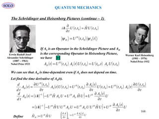
![QUANTUM MECHANICS
SOLO
( ) ( ) ( ) ( ) ( ) ( ) ( ) ( ) ( ) ( )trtprA
t
trtrtprHtprAtprAtprHtr
h
i
tA
td
d
,ˆ|,ˆ,ˆ|,ˆ,ˆ|,ˆ,ˆˆ,ˆ,ˆ,ˆ,ˆ,ˆ,ˆˆ|,ˆ
ψψψψ
∂
∂
+−
/
=
or
( ) [ ] ψψψψ |||ˆ,|
1
A
t
HA
hi
tA
td
d
∂
∂
+
/
=
where Commutator of H and A.[ ] ( ) ( ) ( ) ( )tprAtprHtprHtprAHA ,ˆ,ˆ,ˆ,ˆˆ,ˆ,ˆˆ,ˆ,ˆ:,
−=
We obtain
The previous equation can be written (shorthand notation) as
( ) [ ] A
t
HA
hi
tA
td
d
∂
∂
+
/
= ˆ,
1
Transition from Quantum Mechanics to Classical Mechanics.
171](https://image.slidesharecdn.com/5-introductiontoquantummechanics-sololaptop-150813162751-lva1-app6891/85/5-introduction-to-quantum-mechanics-171-320.jpg)
![QUANTUM MECHANICS
SOLO
( )
( )
∂
∂
−=
∂
∂
=
r
tprH
td
pd
p
tprH
td
rd
,,
,,
In Classical Mechanics the Equation of Motion of a Particle of mass m can be described
Using Hamilton-Jacobi Canonical Equations
Transition from Quantum Mechanics to Classical Mechanics.
where is the Hamiltonian( ) ( )trV
m
pp
tprH ,
2
:,,
+
⋅
=
To see this
( )
( ) ( )
=
∂
∂
−=
∂
∂
−=
==
∂
∂
=
=
F
r
trV
r
tprH
td
pd
m
p
p
tprH
td
rd mp
,,,
v
,, v
For any differentiable function we have( )tprA ,,
( ) ( ) ( ) ( ) ( ) ( ) ( ) ( ) ( )
t
tprA
r
tprH
p
tprA
p
tprH
r
tprA
t
tprA
td
pd
p
tprA
td
rd
r
tprA
tprA
td
d
∂
∂
+
∂
∂
∂
∂
−
∂
∂
∂
∂
=
∂
∂
+
∂
∂
+
∂
∂
=
,,,,,,,,,,,,,,,,
,,
Define Poisson Brackets{ } ( ) ( ) ( ) ( )
r
tprH
p
tprA
p
tprH
r
tprA
HA
∂
∂
∂
∂
−
∂
∂
∂
∂
=
,,,,,,,,
:,
( ) { } ( )
t
tprA
HAtprA
td
d
∂
∂
+=
,,
,,,
Carl Gustav Jacob Jacobi
(1804-1851)
William Rowan Hamilton
(1805-1855)
Siméon Denis
Poisson
1781-1840
172We see that to go from Classical to Quantum we must replace the Poisson Brackets { }with
the Commutator [ ] multiplied by .( )hi //1](https://image.slidesharecdn.com/5-introductiontoquantummechanics-sololaptop-150813162751-lva1-app6891/85/5-introduction-to-quantum-mechanics-172-320.jpg)
![QUANTUM MECHANICS
SOLO
We obtained
Let compute ( ) [ ] ( )
[ ] [ ] [ ]
( )[ ]trVr
him
p
r
hi
trV
m
p
r
hi
r
t
Hr
hi
tr
td
d CBCACBA
,,
1
2
,
1
,
2
,
1ˆ,
1 2,,,2
0
/
+
/
=
+
/
=
∂
∂
+
/
=
+=+
[ ]
[ ] [ ] [ ]
[ ] [ ] p
m
prpppr
him
ppr
himm
p
r
hi hihi
CABCBABCA
1
,,
2
1
,
2
1
2
,
1 ,,,2
=+
/
=⋅
/
=
/ ////
+=
( )[ ] ( ) ( ) 0,,
1
,,
1
=−
/
=
/
rtrVtrVr
hi
trVr
hi
Therefore ( ) ptr
td
d
m
=
( ) [ ] A
t
HA
hi
tA
td
d
∂
∂
+
/
= ˆ,
1
Transition from Quantum Mechanics to Classical Mechanics.
173](https://image.slidesharecdn.com/5-introductiontoquantummechanics-sololaptop-150813162751-lva1-app6891/85/5-introduction-to-quantum-mechanics-173-320.jpg)
![QUANTUM MECHANICS
SOLO
In the same way ( ) [ ] ( )
[ ] [ ] [ ]
( )[ ]trVp
him
pp
p
hi
trV
m
p
p
hi
p
t
Hp
hi
tp
td
d CBCACBA
,,
1
2
,
1
,
2
,
1ˆ,
1 ,,,2
0
/
+
⋅
/
=
+
/
=
∂
∂
+
/
=
+=+
[ ]
[ ] [ ] [ ]
[ ] [ ] 0,,
2
1
,
2
1
00
,,,
=+
/
=⋅
/
+=
pppppp
him
ppp
him
CABCBABCA
( )[ ] ( )[ ] ( )( ) ( )∫∫ ∇+∇−=∇/−
/
=
/
ψψψψ trVrdtrVrdtrVhi
hi
trVp
hi
,,,,
1
,,
1 *3*3
( )( ) ( ) ( ) ( )( ) ( ) FtrVtrVrdtrVrdtrVrdtrVrd
=∇−=∇−=∇+∇−∇−= ∫∫∫∫ ,,,,, *3*3*3*3
ψψψψψψψψ
Therefore ( ) ( ) FtrVtp
td
d
=∇−= ,
Transition from Quantum Mechanics to Classical Mechanics.
174](https://image.slidesharecdn.com/5-introductiontoquantummechanics-sololaptop-150813162751-lva1-app6891/85/5-introduction-to-quantum-mechanics-174-320.jpg)
![QUANTUM MECHANICS
SOLO
Time Independent Hamiltonian
Transition from Quantum Mechanics to Classical Mechanics.
Assume a Time Independent Hamiltonian H
=
∂
∂
0
ˆ
t
H
than choosing in the equationHA ˆ=
( ) [ ] A
t
HA
hi
tA
td
d
∂
∂
+
/
= ˆ,
1
we obtain
( ) [ ] 0ˆˆ,ˆˆ
0
0
=
∂
∂
+
/
=
H
t
HH
h
i
tH
td
d
Since the Total Energy is a Constant of Motion. This is the analogue to
Conservation of Energy in Classical Mechanics.
EH ˆˆ =
( ) ( ) ( )prErV
m
pp
prH
,
2
:, =+
⋅
=
( ) ( ) { } ( ) 0
,
,,,
0
0
=
∂
∂
+==
t
prH
HHprH
td
d
prE
td
d
176](https://image.slidesharecdn.com/5-introductiontoquantummechanics-sololaptop-150813162751-lva1-app6891/85/5-introduction-to-quantum-mechanics-176-320.jpg)
![QUANTUM MECHANICS
SOLO
Virial Theorem
Transition from Quantum Mechanics to Classical Mechanics.
Assume a Time Independent Operator in the equation( ) prprA ˆˆ,
⋅=
( ) [ ]
0
ˆ,
1
A
t
HA
hi
tA
td
d
∂
∂
+
/
=
Assume also a Time Independent Hamiltonian, whose Eigenfunctions are given using
( ) ( ) ( )trEtrprH HnnHn ,,,ˆ
Ψ=Ψ
Schrödinger Equation for |ψ(t)› is ( ) ( ) ( )trprH
h
i
tr
t
HH ,,ˆ,
ψψ
/
−=
∂
∂
( ) ( ) HEertr htEi
HH == /−
,0,, /
ψψ
Using those Eigenfunction we can calculate
( ) ( ) ( ) ( ) ( ) ( )∑∫∑∫ === −
n
HnHn
n
tEi
Hn
tEi
HnHH rprArrderprAerrdAA 0,,0,0,,0,|| *3*3
ψψψψψψ
We can see that if A is not an explicit function of time then <A> is Time Independent
( ) 0=tA
td
d
177](https://image.slidesharecdn.com/5-introductiontoquantummechanics-sololaptop-150813162751-lva1-app6891/85/5-introduction-to-quantum-mechanics-177-320.jpg)
![QUANTUM MECHANICS
SOLO
Virial Theorem
Transition from Quantum Mechanics to Classical Mechanics.
Assume a Time Independent Operator in the equation
[ ] ( ) ( )[ ]rVpr
m
pp
prrV
m
pp
prHpr
,ˆˆ
2
ˆˆ
,ˆˆˆ
2
ˆˆ
,ˆˆˆ,ˆˆ ⋅+
⋅
⋅=
+
⋅
⋅=⋅
[ ] [ ]( ) [ ] [ ] [ ] [ ] m
pp
hipprpprpppprppr
m
pprppppr
mm
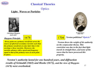
pp
pr
hihi
ˆˆ
ˆˆ,ˆˆ,ˆˆˆˆˆˆ,ˆˆ,ˆˆ
2
1ˆ,ˆˆˆˆˆ,ˆˆ
2
1
2
ˆˆ
,ˆˆ
00
⋅
/=
+⋅+⋅
+=⋅⋅+⋅⋅=
⋅
⋅
//
( )[ ] ( )[ ] ( )[ ] ( )[ ] ( )rVrhirVhirprVrrVprrVpr
∇/−=∇/−=+=⋅ ,ˆ,,ˆˆ,ˆ,ˆ,ˆ,ˆˆ
0
( ) prprA ˆˆ,
⋅=
( ) [ ]
0ˆ,
1
0
=
∂
∂
+
/
= A
t
HA
hi
tA
td
d
We obtain
( )[ ] ( )[ ] ( )( ) ( )( ) ( )( )∫∫∫ ∇/−=∇−∇/−=∇/−=∇/− ψψψψψψ rVrdhirVrdrVrdhirVhirVhi
*3*3*3
,,
[ ] ( ) 0ˆ
2
ˆˆ
2ˆ,ˆˆ =∇⋅/−
⋅
/=⋅ rVrhi
m
pp
hiHpr
T
where we used
( )rVrT
∇⋅=2 Virial Theorem 178
Return to Table of Content](https://image.slidesharecdn.com/5-introductiontoquantummechanics-sololaptop-150813162751-lva1-app6891/85/5-introduction-to-quantum-mechanics-178-320.jpg)
![08/13/15 187
SOLO
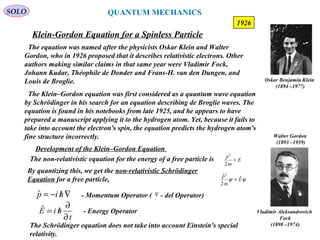
Non-relativistic Schrödinger Equation in an Electromagnetic Field
Electromagnetic Field
In Quantum Mechanics an electron, with no external electromagnetic field presented, is
expressed by a wave function ψ that satisfies the Schrödinger Equation:
( ) ( ) ( )rtprH
t
rt
hi
,,
,
ψ
ψ
=
∂
∂
/
( ) ( ) ( )rV
m
rtp
prH
+=
2
,
:,
2
where Hamiltonian
and is Canonical Momentum, and is represented by the differential operatorp
∇/−= hipˆ - Momentum Operator ( - del Operator)∇
The Schrödinger Equation:
( ) ( ) ( )rtVrt
m
h
t
rt
hi
,,
2
, 2
2
ψψ
ψ
+∇
/
−=
∂
∂
/
AB
t
A
c
E
×∇=∇−
∂
∂
−= ,
1
ϕIf an external Electromagnetic Field :
is presented, we must replace
BE
,
ϕeVVA
c
e
pp +→−→ &
( ) ( ) ( ) ( ) ( )[ ] ( )rtrterVrt
c
rtA
h
ei
m
h
t
rt
hi
,,,
,
2
,
2
2
ψϕψ
ψ
++
/
−∇
/
−=
∂
∂
/
Schrödinger Equation in
an Electromagnetic Field
( )
( ) ( )
( ) ( )rterV
m
rtA
c
e
rtp
prH
,
2
,,
:,
2
ϕ++
−
=
to obtain Non-relativistic Hamiltonian in
an Electromagnetic Field](https://image.slidesharecdn.com/5-introductiontoquantummechanics-sololaptop-150813162751-lva1-app6891/85/5-introduction-to-quantum-mechanics-187-320.jpg)
![08/13/15 188
SOLO
Electromagnetic Field
( ) ( ) ( ) ( ) ( )[ ] ( )rtrterVrtrtA
c
e
i
h
mt
rt
hi
,,,,
2
1,
2
ψϕψ
ψ
++
−∇
/
=
∂
∂
/ Schrödinger Equation in
an Electromagnetic Field
xi
h
p
∂
∂/
=:ˆUsing the Momentum Operator we can write
( ) ( ) ( ) ( ) ( )rtrterVrtA
c
e
p
mt
rt
hi
,,,ˆ
2
1,
2
ψϕ
ψ
++
−=
∂
∂
/
Schrödinger Equation in
an Electromagnetic Field
Non-relativistic Schrödinger Equation in an Electromagnetic Field
Return to Table of Content](https://image.slidesharecdn.com/5-introductiontoquantummechanics-sololaptop-150813162751-lva1-app6891/85/5-introduction-to-quantum-mechanics-188-320.jpg)
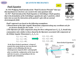

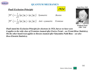
![Pauli Equation
SOLO
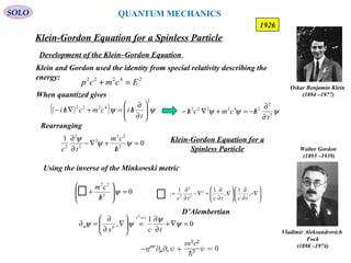
Pauli Equation or Schrödinger–Pauli equation is the formulation of the
Schrödinger equation for spin-½ particles, which takes into account the
interaction of the particle's spin with an external electromagnetic field. It is the
non-relativistic limit of the Dirac equation and can be used where particles are
moving at speeds much less than the speed of light, so that relativistic effects can
be neglected. It was formulated by Wolfgang Pauli in 1927.
193
1927
( ) ( ) ( ) ( ) ( )rtrterVrtA
c
e
p
mt
rt
hi
,,,ˆ
2
1,
2
ψϕ
ψ
++
−=
∂
∂
/
Schrödinger Equation in an
Electromagnetic Field
for a spinless particle
For a particle of mass m, charge e, and without spin, in an electromagnetic field described
by the vector potential A = (Ax, Ay, Az) and scalar electric potential φ, and in a conservative
external field described by the potential ,the Schrödinger equation is:( )rV
where σ = (σx, σy, σz) are the Pauli matrices collected into a tensor for convenience, p = −iħ is∇
the momentum operator wherein denotes the gradient operator, and∇
is the two-component Spinor Wave Function, a column vector written in Dirac notation.
=
−
+
2/1
2/1
1x2
ψ
ψ
ψ
( ) ( ) ( ) ( )[ ] ( )rtrterVIrtA
c
e
p
mt
rt
hi
,,,ˆ
2
1,
2x2
2
ψϕσ
ψ
++
−⋅=
∂
∂
/
Pauli- Schrödinger Equation in an
Electromagnetic Field for a particle
with Spin 2/h/±
For a particle of mass m ,charge e, spin in an electromagnetic field described by the
vector potential A = (Ax, Ay, Az) and scalar electric potential , and scalar electric potential ,ϕ ϕ
and in a conservative external field described by the potential ,the Pauli equation is:( )rV
2/h/±
Wolfgang Pauli
1900 - 1958
Nobel Prize 1945
QUANTUM MECHANICS](https://image.slidesharecdn.com/5-introductiontoquantummechanics-sololaptop-150813162751-lva1-app6891/85/5-introduction-to-quantum-mechanics-193-320.jpg)
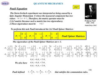
![Pauli Equation
SOLO
194
The Hamiltonian operator is
is a 2 × 2 matrix operator, because of the Pauli matrices. Substitution into the
Schrödinger equation
gives the Pauli equation.
1927
ψψ EH ˆˆ =
( ) ( ) ( )[ ]
++
−⋅= rterVIrtA
c
e
p
m
H
,,ˆ
2
1
:ˆ
2x2
2
2x2 ϕσ
t
IhiE
∂
∂
/= 2x22x2 :ˆ
The Pauli matrices can be removed from the kinetic energy term, using the Pauli vector
identity:
Let develop
( )( ) ( ) ( )21222121
ˆˆˆˆˆˆ nniInnnn x ×⋅+⋅=⋅⋅ σσσ
( ) ( ) ( ) ( )
( )
( ) ( )
( )
( ) ( )
i
hp
AA
pAeipAeApeiApe
pp
i
hAA
i
h
c
e
iA
c
e
pA
c
e
p
AA
c
e
pA
c
e
Ap
c
e
ppA
c
e
p
∇
/=
⋅
×⋅+⋅×⋅+⋅
⋅
∇
/×+×
∇
/⋅−
−⋅
−=
⋅⋅⋅
+⋅⋅⋅−⋅⋅⋅−⋅⋅⋅=
−⋅
ˆ
2
ˆˆˆˆ
ˆˆ
2
ˆˆ
ˆˆˆˆˆ
σ
σσσσσσσσσ
σσ
Wolfgang Pauli
1900 - 1958
Nobel Prize 1945
QUANTUM MECHANICS](https://image.slidesharecdn.com/5-introductiontoquantummechanics-sololaptop-150813162751-lva1-app6891/85/5-introduction-to-quantum-mechanics-194-320.jpg)
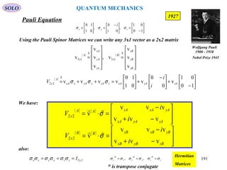
![Pauli Equation
SOLO
195
where B = × A is the magnetic field.∇
( ) ( ) ( ) ( ) ( )[ ] ( )
( ) ( ) ( ) ( )( ) ( ) ( )[ ] ( )rtrterVIrtArtAh
c
e
rtA
c
e
rtp
m
rtrterVIrtA
c
e
rtp
mt
rt
hi
,,,,,,ˆ
2
1
,,,,ˆ
2
1,
2x2
2
2x2
2
ψϕσ
ψϕσ
ψ
++
∇×+×∇⋅/−
−=
++
−⋅=
∂
∂
/
Pauli- Schrödinger Equation in an Electromagnetic Field for a particle
with Spin 2/h/±
( ) ( )( ) ( ) ( ) ( )[ ] ( ) ( )
( ) ( ) ( ) ( ) ( ) ( )rtrtArtArtrtArt
rtrtArtrtArtrtArtA
,,,,,,
,,,,,,,
ψψψ
ψψψ
∇×+×∇+×∇=
∇×+×∇=∇×+×∇
( ) ( ) ( ) ( ) ( ) ( )[ ] ( )rtrterVIrtB
cm
he
rtA
c
e
rtp
mt
rt
hi
,,,
2
,,ˆ
2
1,
2x2
2
ψϕσ
ψ
++⋅
/
−
−=
∂
∂
/
Pauli- Schrödinger Equation in an Electromagnetic Field for a particle with Spin 2/h/±
and the Hamiltonian is
( ) ( ) ( ) ( ) ( ) ( )[ ]rterVIrtB
cm
he
rtA
c
e
rtp
m
rtH
,,
2
,,ˆ
2
1
:, 2x2
2
ϕσ ++⋅
/
−
−=
( ) ( ) ( ) ( )rtBrtrtArt
,,,, ψψ =×∇=
Wolfgang Pauli
1900 - 1958
Nobel Prize 1945
1927
QUANTUM MECHANICS](https://image.slidesharecdn.com/5-introductiontoquantummechanics-sololaptop-150813162751-lva1-app6891/85/5-introduction-to-quantum-mechanics-195-320.jpg)
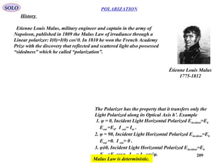
![204
Dirac Equation
SOLO
1928
Ψ=Ψ
−∇/−⋅−
−
∂
∂
/ cmA
c
e
hi
c
e
x
hi
γϕγ
0
0
Dirac Equation
Let multiply this equation by and using0
γ
c
4x4
2x2
2x2
2x2
2x200
0
0
0
0
I
I
I
I
I
=
−
−
=γγ
=
−
−
=
0
0
0
0
0
0
2x2
2x20
σ
σ
σ
σ
γγ
I
I
we obtain
( )
Ψ=Ψ
−∇/−⋅−
−
∂
∂
/ 02000
γγγϕγγ
cmA
c
e
hic
c
e
tc
hic
rearranging we obtain
( )[ ] Ψ=Ψ++−∇/−⋅=Ψ
∂
∂
/ 4x4
20000 ˆHcmeAehci
t
hi γϕγγγγ
where the 4x4 Hamiltonian is defined as
( )[ ]20000
4x4 :ˆ cmeAehciH γϕγγγγ
++−∇/−⋅=
( )
( )
=Ψ
1x2
1x2
:1x4 B
A
ψ
ψ
Paul Adrien Maurice
Dirac
(1902 – 1984)
Nobel Prize 1933
QUANTUM MECHANICS](https://image.slidesharecdn.com/5-introductiontoquantummechanics-sololaptop-150813162751-lva1-app6891/85/5-introduction-to-quantum-mechanics-204-320.jpg)

![QUANTUM MECHANICS
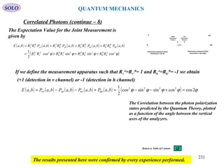
Copenhagen Interpretation of Quantum Mechanics
The Copenhagen interpretation is one of the earliest and most commonly taught
interpretations of quantum mechanics.[1]
It holds that quantum mechanics does not yield
a description of an objective reality but deals only with probabilities of observing, or
measuring, various aspects of energy quanta, entities that fit neither the classical idea of
particles nor the classical idea of waves. The act of measurement causes the set of
probabilities to immediately and randomly assume only one of the possible values. This
feature of the mathematics is known as wavefunction collapse. The essential concepts of
the interpretation were devised by Niels Bohr, Werner Heisenberg and others in the years
1924–27.
There are several basic principles that are generally accepted as being part of the
interpretation:
1. A system is completely described by a wave function Ψ, representing the state of the
system, which evolves smoothly in time, except when a measurement is made, at which
point it instantaneously collapses to an eigenstate of the observable that is measured.
2. The description of nature is essentially probabilistic, with the probability of a given
outcome of a measurement given by the square of the modulus of the amplitude of the
wave function. (The Born rule, after Max Born)
SOLO
233](https://image.slidesharecdn.com/5-introductiontoquantummechanics-sololaptop-150813162751-lva1-app6891/85/5-introduction-to-quantum-mechanics-233-320.jpg)


![Nathan Rosen
(1909-1995)
Boris Yakovlevich
Podolsky
(1896–1966)
Albert Einstein
(/1879 – 1955)
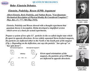
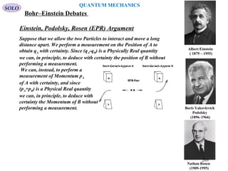
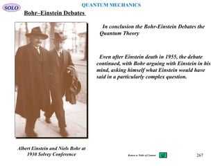
Einstein, Podolsky, Rosen (EPR) Argument
Let denote the two Particles by A and B.
The Position qA and Momentum pA of Particle A are complementary
observables and we cannot measure one without introducing an
uncertainty in the other according to Heisenberg Uncertainty Principle.
Similar for qB and pB of Particle B.
SOLO
[ ] [ ] hipqpq BBAA /== ˆ,ˆˆ,ˆ
Since A and B are different
Quantum Particles we also have
[ ] [ ] 0ˆ,ˆˆ,ˆ == ABBA pqpq
Now consider the quantities BABA ppPqqQ ˆˆ:ˆ&ˆˆ:ˆ +=−=
Let compute the Commutator
[ ] ( )( ) ( )( )
( )
( ) ( ) ( ) ( )
[ ] [ ] [ ] [ ] 0ˆ,ˆˆ,ˆˆ,ˆˆ,ˆ
ˆˆˆˆˆˆˆˆˆˆˆˆˆˆˆˆ
ˆˆˆˆˆˆˆˆˆˆˆˆˆˆˆˆ
ˆˆˆˆˆˆˆˆˆˆˆˆˆ,ˆ
00
=−−+=
−−−−−+−=
−+−−−−+=
−+−+−=−=
//
hi
BBABBA
hi
AA
BBBBBAABABBAAAAA
BBABBAAABBABBAAA
BABABABA
pqpqpqpq
qppqqppqqppqqppq
qpqpqpqppqpqpqpq
qqppppqqQPPQPQ
Hence , the Operators commute, therefore we can
measure the Difference between Positions of Particles A and B and the
Sum of their Moments with high precision. Q and P are therefore
Physically Real Quantities.
[ ] 0ˆ,ˆ =PQ PandQ ˆˆ
QUANTUM MECHANICS
Bohr–Einstein Debates
262](https://image.slidesharecdn.com/5-introductiontoquantummechanics-sololaptop-150813162751-lva1-app6891/85/5-introduction-to-quantum-mechanics-262-320.jpg)
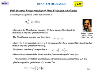
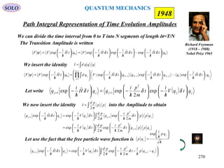
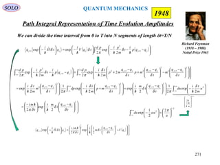
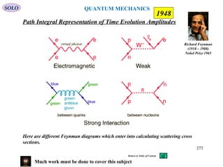
![Path Integral Representation of Time Evolution Amplitudes
SOLO
The Path Integral approach to Quantum Mechanics was developed by Feynman in 1948.
Richard Feynman
(1918 – 1988)
Nobel Prize 1965
The Path Integral formulation of Quantum Mechanics is a description
of Quantum Theory which generalizes the Action Principle of Classical
Mechanics. It replaces the classical notion of a single, unique trajectory
for a system with a sum, or functional integral, over an infinity of
possible trajectories to compute a quantum amplitude.
The basic idea of the path integral formulation can be traced back to Norbert Wiener,
who introduced the Wiener integral for solving problems in diffusion and Brownian
motion.[1]
This idea was extended to the use of the Lagrangian in quantum mechanics by P.
A. M. Dirac in his 1933 paper.[2]
The complete method was developed in 1948 by Richard
Feynman. Some preliminaries were worked out earlier, in the course of his doctoral thesis
work with John Archibald Wheeler. The original motivation stemmed from the desire to
obtain a quantum-mechanical formulation for the Wheeler–Feynman absorber theory
using a Lagrangian (rather than a Hamiltonian) as a starting point.
1948QUANTUM MECHANICS
268](https://image.slidesharecdn.com/5-introductiontoquantummechanics-sololaptop-150813162751-lva1-app6891/85/5-introduction-to-quantum-mechanics-268-320.jpg)
![Path Integral Representation of Time Evolution Amplitudes
SOLO
Richard Feynman
(1918 – 1988)
Nobel Prize 1965
1948
The Transition Amplitude for the entire time period is
( )∏ ∑∫
−
=
−
=
+
−
−
/
/−
=
/
−=
1
1
1
0
2
1
2
0
2
1
exp
2
ˆexp
N
j
N
j j
jj
j
N
qV
t
qq
mt
h
i
qd
t
hmi
qtH
h
i
FF
δ
δ
δπ
ψ
By taking the limit of large N the Transition Amplitude reduces to
( )∫
/
=
/
−= S
h
i
tqDqtH
h
i
FF expˆexp 0ψ
( ) ( )[ ]∫=
T
tqtqLtdS
0
, where S is the classical action given by
and L is the classical Lagrangian given by ( ) ( )[ ] ( )qVqmtqtqL −= 2
2
1
,
Any possible path of the particle, going from the initial state to the final state, is
approximated as a broken line and included in the measure of the integral
( ) ( )∏ ∫∫
−
=∞→
/
−
=
1
1
2
2
lim
N
j j
N
N
qd
th
mi
tqD
δπ
This expression actually defines the manner in which the path integrals are to be taken.
The coefficient in front is needed to ensure that the expression has the correct dimensions,
but it has no actual relevance in any physical application.
QUANTUM MECHANICS
272](https://image.slidesharecdn.com/5-introductiontoquantummechanics-sololaptop-150813162751-lva1-app6891/85/5-introduction-to-quantum-mechanics-272-320.jpg)
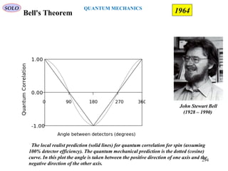
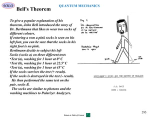
![Bell's Theorem
Bell considers the same experiment but focuses on correlations
between results of spin measurement at different orientation of the two
magnets.
He then shows that the correlations predicted by quantum mechanics
cannot be generated by local hidden parameters:
Quantum mechanics => There can't be local hidden parameters.
Bell:
Together with the EPR argument, this entails that either quantum mechanics makes wrong
predictions or locality does not hold. Since (most of) the experiments confirm the quantum
prediction, we conclude:
Bell + EPR + experiment=>Nature is nonlocal. There is instantaneous action-at-a-distance
Oct 15, 1997. Written by students of the Bohmian mechanics group.
http://www.mathematik.uni-muenchen.de/~bohmmech/Poster/post/postE.html
John Stewart Bell
(1928 – 1990)
Bell's theorem, derived in his seminal 1964 paper titled On the Einstein
Podolsky Rosen paradox,[5]
has been called, on the assumption that the
theory is correct, "the most profound in science".[11]
Perhaps of equal
importance is Bell's deliberate effort to encourage and bring legitimacy to
work on the completeness issues, which had fallen into disrepute
http://en.wikipedia.org/wiki/Bell%27s_theorem
John Stewart Bell, "On the Einstein-Podolsky-Rosen paradox", Physics 1, (1964) 195-200. Reprinted
in Speakable and Unspeakable in Quantum Mechanics, Cambridge University Press, 2004.
SOLO
1964
289
QUANTUM MECHANICS](https://image.slidesharecdn.com/5-introductiontoquantummechanics-sololaptop-150813162751-lva1-app6891/85/5-introduction-to-quantum-mechanics-289-320.jpg)
![Bell's Theorem
SOLO
1964
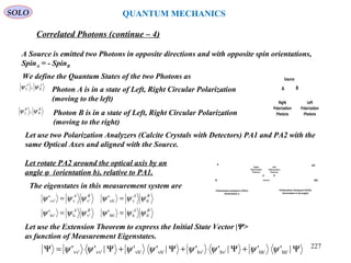
Bell considered three theoretical experiences with correlated photons. In each experience
a Source emitted two correlated photons in two opposite directions to two optical aligned
Polarization Analyzers PA1 and PA2. The Polarization Analyzers PA1 and PA2, in those
experiments are in three possible orientations
(a)φ = 0º
(b)φ = 22.5º
(c)φ = 45º
Source
v͛
h͛
Polarization Analyzer2 (PA2)
Orientation b (ϕ =22.5)
v
h
Polarization Analyzer1 (PA1)
Orientation a (ϕ=0)
BA
Left
Polarization
Photons
Right
Polarization
Photons
Experience 1
Source
v͛͛
h͛͛
Polarization Analyzer2 (PA2)
Orientation c (ϕ =45)
v
h
Polarization Analyzer1 (PA1)
Orientation a (ϕ=0)
BA
Left
Polarization
Photons
Right
Polarization
Photons
Experience2
Source
v͛͛
h͛͛
Polarization Analyzer2 (PA2)
Orientation c (ϕ =45)
v
h
Polarization Analyzer1 (PA1)
Orientation b (ϕ=22.5)
BA
Left
Polarization
Photons
Right
Polarization
Photons
Experience 3
Bell’s Theorem checks the validity of EPR conjunction that the to explain the entanglement of
quantum particle, there must exist locally hidden variables that communicate between the
entangled particles at speeds less than speed of light.
Let perform the same large number M of experiments 1, 2 and 3 and for each orientation (a),
(b) and (c) count the separately the detections in Vertical (v) and Horizontal (h) channels.
Let define
N [av], N[ah] - Number of detections in v channels, and in h channels in (a) orientation in
experiments 1 and 2
N [bv], N[bh] - Number of detections in v channels, and in h channels in (b) orientation in
experiments 1 and 3
N [cv], N[ch] - Number of detections in v channels, and in h channels in (c) orientation in
290
QUANTUM MECHANICS](https://image.slidesharecdn.com/5-introductiontoquantummechanics-sololaptop-150813162751-lva1-app6891/85/5-introduction-to-quantum-mechanics-290-320.jpg)
![Bell's Theorem
SOLO
1964
Source
v͛
h͛
Polarization Analyzer2 (PA2)
Orientation b (ϕ =22.5)
v
h
Polarization Analyzer1 (PA1)
Orientation a (ϕ=0)
BA
Left
Polarization
Photons
Right
Polarization
Photons
Experience 1
Source
v͛͛
h͛͛
Polarization Analyzer2 (PA2)
Orientation c (ϕ =45)
v
h
Polarization Analyzer1 (PA1)
Orientation a (ϕ=0)
BA
Left
Polarization
Photons
Right
Polarization
Photons
Experience2
Source
v͛͛
h͛͛
Polarization Analyzer2 (PA2)
Orientation c (ϕ =45)
v
h
Polarization Analyzer1 (PA1)
Orientation b (ϕ=22.5)
BA
Left
Polarization
Photons
Right
Polarization
Photons
Experience 3
Since in the 3 experiments we have two Polarizations Analyzers in the same orientation, and
since we assume that each photon will be detected in the Vertical v or the Horizontal h channel,
and we perform M measurements in each experience we ca write
[ ] [ ] [ ] [ ] [ ] [ ] McNcNbNbNaNaN 2hvhvhv =+=+=+
For large number of M measurements we can write
[ ] [ ] [ ] [ ]
M
aN
aP
M
aN
aP
MM 2
lim,
2
lim h
h
v
v
∞→∞→
== Probabilities of detections in v channels, and in h
channels in (a) orientation in experiments 1 and 2
[ ] [ ] [ ] [ ]
M
bN
bP
M
bN
bP
MM 2
lim,
2
lim h
h
v
v
∞→∞→
== Probabilities of detections in v channels, and in h
channels in (b) orientation in experiments 1 and 3
[ ] [ ] [ ] [ ]
M
cN
cP
M
cN
cP
MM 2
lim,
2
lim h
h
v
v
∞→∞→
== Probabilities of detections in v channels, and in h
channels in (c) orientation in experiments 2 and 3
291
QUANTUM MECHANICS](https://image.slidesharecdn.com/5-introductiontoquantummechanics-sololaptop-150813162751-lva1-app6891/85/5-introduction-to-quantum-mechanics-291-320.jpg)
![Bell's Theorem
SOLO
1964
Source
v͛
h͛
Polarization Analyzer2 (PA2)
Orientation b (ϕ =22.5)
v
h
Polarization Analyzer1 (PA1)
Orientation a (ϕ=0)
BA
Left
Polarization
Photons
Right
Polarization
Photons
Experience 1
Source
v͛͛
h͛͛
Polarization Analyzer2 (PA2)
Orientation c (ϕ =45)
v
h
Polarization Analyzer1 (PA1)
Orientation a (ϕ=0)
BA
Left
Polarization
Photons
Right
Polarization
Photons
Experience2
Source
v͛͛
h͛͛
Polarization Analyzer2 (PA2)
Orientation c (ϕ =45)
v
h
Polarization Analyzer1 (PA1)
Orientation b (ϕ=22.5)
BA
Left
Polarization
Photons
Right
Polarization
Photons
Experience 3
Since we assume local reality, the measurements in the orientations (a), (b) and (c) are
independent, therefore we can write
P [av,bh] = P [av]* P[bh] - Probability of joint detections in v channel in (a) orientation and in
h channel in (b) orientations in all 3 experiments.
P [bv,ch] = P [bv]* P[ch] - Probability of joint detections in v channel in (b) orientation and in
h channel in (c) orientations in all 3 experiments.
P [av,ch] = P [abv]* P[ch] - Probability of joint detections in v channel in (a) orientation and in
h channel in (c) orientations in all 3 experiments.
Also
[ ] [ ] [ ] [ ]( ) [ ] [ ]vhvhhv
1
vhhvhv ,,,,,, cbaPcbaPcPcPbaPbaP +=+⋅=
[ ] [ ] [ ] [ ]( ) [ ] [ ]hhvhvvhvhvhv ,,,,,, cbaPcbaPbPbPcaPcaP +=+=
[ ] [ ] [ ] [ ]( ) [ ] [ ]hvhhvvhvhvhv ,,,,,, cbaPcbaPaPaPcbPcbP +=+⋅=
[ ] [ ]hhvhv ,,, cbaPbaP ≥
[ ] [ ]hvvhv ,,, cbaPcbP ≥
[ ] [ ] [ ] [ ]
[ ]
[ ]hv
,
hvvhhvhvhv ,,,,,,,
hv
caPcbaPcbaPcbPbaP
caP
=
+≥+
292
QUANTUM MECHANICS](https://image.slidesharecdn.com/5-introductiontoquantummechanics-sololaptop-150813162751-lva1-app6891/85/5-introduction-to-quantum-mechanics-292-320.jpg)
![Bell's Theorem
SOLO
1964
Source
v͛
h͛
Polarization Analyzer2 (PA2)
Orientation b (ϕ =22.5)
v
h
Polarization Analyzer1 (PA1)
Orientation a (ϕ=0)
BA
Left
Polarization
Photons
Right
Polarization
Photons
Experience 1
Source
v͛͛
h͛͛
Polarization Analyzer2 (PA2)
Orientation c (ϕ =45)
v
h
Polarization Analyzer1 (PA1)
Orientation a (ϕ=0)
BA
Left
Polarization
Photons
Right
Polarization
Photons
Experience2
Source
v͛͛
h͛͛
Polarization Analyzer2 (PA2)
Orientation c (ϕ =45)
v
h
Polarization Analyzer1 (PA1)
Orientation b (ϕ=22.5)
BA
Left
Polarization
Photons
Right
Polarization
Photons
Experience 3
Bell's Inequality[ ] [ ] [ ]hvhvhv ,,, caPcbPbaP ≥+
For chosen
(a) φ = 0º
(b) φ = 22.5º
(c) φ = 45º
( ) ( )abbaP −∠== ϕϕ,sin
2
1
, 2
hv'Using Quantum Theory we found
( ) ( ) ( )
45sin
2
1
5.22sin
2
1
5.22sin
2
1 222
≥+
or which is incorrect2500.01464.0 ≥
Quantum Theory is incompatible with any Local Hidden Variable Theory.
Conclusion of Bell's Inequality
There is more than one Inequality that are collectively known as Bell's Inequality.
All of them give the same conclusion. 293
QUANTUM MECHANICS](https://image.slidesharecdn.com/5-introductiontoquantummechanics-sololaptop-150813162751-lva1-app6891/85/5-introduction-to-quantum-mechanics-293-320.jpg)
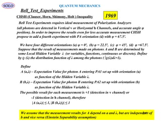
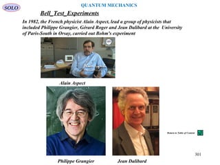
![Bell_Test_Experiments
SOLO
John Francis Clauser
Born 1942
CHSH (Clauser, Horn, Shimony, Holt ) Inequality
Abner Shimony
Born 1928
CHSH inequality can be used in the proof of Bell's theorem, which
states that certain consequences of entanglement in quantum
mechanics cannot be reproduced by local hidden variable theories.
Experimental verification of violation of the inequalities is seen as
experimental confirmation that nature cannot be described by local
hidden variables theories. CHSH stands for John Clauser, Michael
Horne, Abner Shimony and Richard Holt, who described it in a
much-cited paper published in 1969 (Clauser et al., 1969).[1]
They
derived the CHSH inequality, which, as with John Bell’s original
inequality (Bell, 1964),[2]
is a constraint on the statistics of
"coincidences" in a Bell test experiment which is necessarily true if
there exist underlying local hidden variables (local realism). This
constraint can, on the other hand, be infringed by quantum
mechanics
Richard Holt
Michael Horne
1969
296
QUANTUM MECHANICS](https://image.slidesharecdn.com/5-introductiontoquantummechanics-sololaptop-150813162751-lva1-app6891/85/5-introduction-to-quantum-mechanics-296-320.jpg)
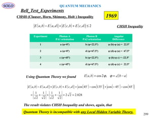
![Bell_Test_Experiments
SOLO
CHSH (Clauser, Horn, Shimony, Holt ) Inequality 1969
The expectation value for the joint measurement of A and B is
E (a,b,λ) = A (a,λ) B (b,λ)
Let average tis result over all Hidden Variable λ, by performing enough
measurements to cover all values of λ.
( ) ( ) ( ) ( )∫ ⋅⋅⋅= λλρλλ dbBaAbaE ,,,
We also can write
( ) ( ) ( ) ( ) ( ) ( )[ ] ( )
( ) ( ) ( )[ ] ( )∫
∫
⋅⋅−⋅=
⋅⋅⋅−⋅=−
λλρλλλ
λλρλλλλ
ddBbBaA
ddBaAbBaAdaEbaE
,,,
,,,,,,
Since |A (a,λ)| ≤ 1 we have
( ) ( ) ( ) ( ) ( )∫ ⋅⋅−≤− λλρλλ ddBbBdaEbaE ,,,,
Similarly ( ) ( ) ( ) ( ) ( )∫ ⋅⋅+≤+ λλρλλ ddBbBdcEbcE ,,,,
Combining those two equations we obtain
( ) ( ) ( ) ( ) ( ) ( ) ( ) ( )[ ] ( )∫ ⋅⋅−+−≤++− λλρλλλλ ddBbBdBbBdcEbcEdaEbaE ,,,,,,,,
Since |B (b,λ)| ≤ 1 we have ( ) ( ) ( ) ( ) 2,,,, ≤−+− λλλλ dBbBdBbB
( ) ( ) ( ) ( ) ( ) 22,,,,
1
=⋅≤++− ∫
λλρ ddcEbcEdaEbaE CHSH Inequality
298
QUANTUM MECHANICS](https://image.slidesharecdn.com/5-introductiontoquantummechanics-sololaptop-150813162751-lva1-app6891/85/5-introduction-to-quantum-mechanics-298-320.jpg)
![Bell_Test_Experiments
SOLO
Alain Aspect (Born 1947)
on a visit to Tel Aviv
University in 2010
Scheme for 1981 Experiment, P's polarisers and D's
detectors. Polariser axes are at angles a and b
respectively.
The diagram shows a typical optical experiment of the two-channel
kind for which Alain Aspect set a precedent in 1982.[2]
Coincidences
(simultaneous detections) are recorded, the results being categorised
as '++', '+−', '−+' or '−−' and corresponding counts accumulated.
Scheme of a "two-channel" Bell test
The source S produces pairs of "photons", sent in opposite directions. Each photon
encounters a two-channel polariser whose orientation can be set by the experimenter.
Emerging signals from each channel are detected and coincidences counted by the
coincidence monitor CM.
In 1982, a group led by, the French physicist Alain Aspect at the University
of Paris-South, carried out Bohm's experiment, demonstrating once and
for all that quantum mechanics does indeed require spooky action. (The
reason that nonlocality does not violate the theory of relativity is that one
cannot exploit it to transmit information faster than light or
instantaneously.)
1982
300
QUANTUM MECHANICS](https://image.slidesharecdn.com/5-introductiontoquantummechanics-sololaptop-150813162751-lva1-app6891/85/5-introduction-to-quantum-mechanics-300-320.jpg)

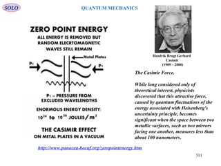
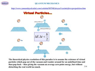
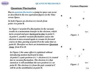
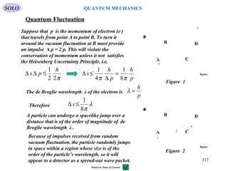
![Quantum Fluctuation
In quantum physics, a quantum vacuum fluctuation (or quantum fluctuation or vacuum
fluctuation) is the temporary change in the amount of energy in a point in space,[1]
arising
from Werner Heisenberg's uncertainty principle.
According to one formulation of the principle, energy and time can be related by the relation
That means that conservation of energy can appear to be violated, but only for small times.
This allows the creation of particle-antiparticle pairs of virtual particles. The effects of
these particles are measurable, for example, in the effective charge of the electron,
different from its "naked" charge.
SOLO
315
QUANTUM MECHANICS
Quantum theory is different from classical theory. The difference is in accounting for the
inner workings of subatomic processes. Classical physics cannot account for such. It was
pointed out by Heisenberg that what "actually" or "really" occurs inside such subatomic
processes as collisions is not directly observable and no unique and physically definite
visualization is available for it. Quantum mechanics has the specific merit of by-passing
speculation about such inner workings. It restricts itself to what is actually observable and
detectable. Virtual particles are conceptual devices that in a sense try to by-pass
Heisenberg's insight, by offering putative or virtual explanatory visualizations for the
inner workings of subatomic processes.](https://image.slidesharecdn.com/5-introductiontoquantummechanics-sololaptop-150813162751-lva1-app6891/85/5-introduction-to-quantum-mechanics-315-320.jpg)
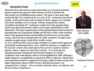
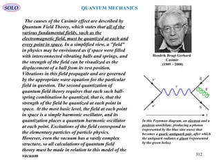
![Quantum Foam
Quantum foam (also referred to as space time foam) is a concept in quantum mechanics devised by John
Wheeler in 1955. The foam is supposed to be conceptualized as the foundation of the fabric of the
universe.[1]
Additionally, quantum foam can be used as a qualitative description of subatomic space time turbulence
at extremely small distances (on the order of the Planck length). At such small scales of time and space,
the Heisenberg uncertainty principle allows energy to briefly decay into particles and antiparticles and
then annihilate without violating physical conservation laws. As the scale of time and space being
discussed shrinks, the energy of the virtual particles increases. According to Einstein's theory of general
relativity, energy curves space time. This suggests that—at sufficiently small scales—the energy of these
fluctuations would be large enough to cause significant departures from the smooth space time seen at
larger scales, giving space time a "foamy" character
Quantum foam is theorized to be the 'fabric' of the Universe, but however cannot be observed yet
because it is just too small. Also, quantum foam is theorized to be created by virtual particles of very
high energy. Virtual particles appear in quantum field theory, arising briefly and then annihilating
during particle interactions in such a way that they affect the measured outputs of the interaction,
even though the virtual particles are themselves space. These "vacuum fluctuations" affect the
properties of the vacuum, giving it a nonzero energy known as vacuum energy, itself a type of zero-
point energy. However, physicists are uncertain about the magnitude of this form of energy.[8]
The Casimir effect can also be understood in terms of the behavior of virtual particles in the empty
space between two parallel plates. Ordinarily, quantum field theory does not deal with virtual
particles of sufficient energy to curve spacetime significantly, so quantum foam is a speculative
extension of these concepts which imagines the consequences of such high-energy virtual particles at
very short distances and times.
SOLO
319
QUANTUM MECHANICS
Return to Table of Content](https://image.slidesharecdn.com/5-introductiontoquantummechanics-sololaptop-150813162751-lva1-app6891/85/5-introduction-to-quantum-mechanics-319-320.jpg)
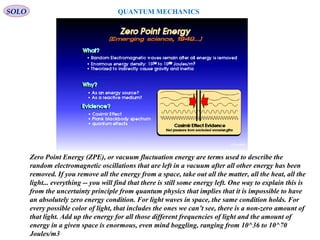
![QUANTUM MECHANICS
SOLO
Interpretation of Quantum Mechanics
330
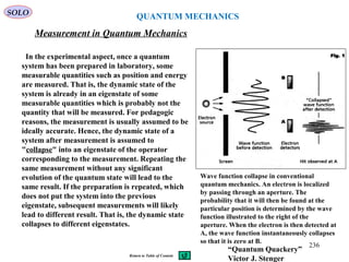
The experiments are done by performing measurements, in which quantum particles are involved.
Those quantum particles (atoms, photon, electrons, protons, neutrons, …) have energy that can be
detected.
• The lest expensive measurements are those with photons (electromagnetic spectrum) that can be
performed in labs with, relatively, non expensive instruments.
• Other experiments are performed by analyzing cosmic rays.
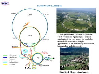
Feynman said, the hadron-hadron work [in the Stanford Linear Acceleration Center
SLAC] was like trying to figure out a pocket watch by smashing two of them together
and watching the pieces fly out.
“Genius: The Life and Science of Richard Feynman” by James Gleick, 1992
Cosmic rays are immensely high-energy radiation, mainly originating outside the Solar
System. They may produce showers of secondary particles that penetrate and impact the
Earth's atmosphere and sometimes even reach the surface. Composed primarily of high-
energy protons and atomic nuclei.
• The most expensive experiments (Particles Collider Facilities), where high energy
particles are smashed. The results of this process (energy scattering) are analyzed to
detect new quantum effects.](https://image.slidesharecdn.com/5-introductiontoquantummechanics-sololaptop-150813162751-lva1-app6891/85/5-introduction-to-quantum-mechanics-330-320.jpg)


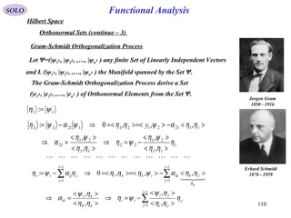
![•Quantity v
•t
•e
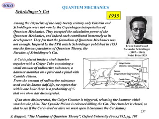
Symbol Value[7][8]
Relative
Standard
Uncertainty
speed of light in vacuum 299 792 458 m·s−1
defined
Newtonian constant of
gravitation
6.67384(80)×10−11
m3
·kg
−1
·s−2 1.2 × 10⁻⁴
Planck constant
6.626 069 57(29) × 10−34
J·s
4.4 × 10⁻⁸
reduced Planck constant
1.054 571 726(47) ×
10−34
J·s
4.4 × 10⁻⁸
Table of universal constants
SOLO
350](https://image.slidesharecdn.com/5-introductiontoquantummechanics-sololaptop-150813162751-lva1-app6891/85/5-introduction-to-quantum-mechanics-350-320.jpg)
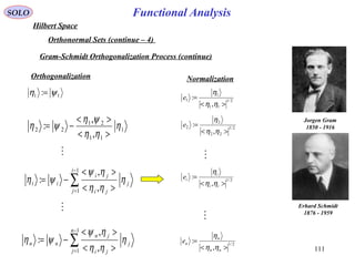
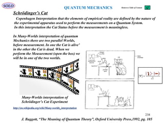
![Table of electromagnetic constants
•Quantity v
•t
•e
Symbol Value[7][8]
(SI units)
Relative Standard
Uncertainty
magnetic constant
(vacuum permeability)
4π × 10−7
N·A−2
= 1.256 637 061... ×
10−6
N·A−2 defined
electric constant (vacuum
permittivity)
8.854 187 817... × 10−12
F·m−1
defined
characteristic impedance
of vacuum
376.730 313 461... Ω defined
Coulomb's constant 8.987 551 787... × 109
N·m²·C−2
defined
elementary charge 1.602 176 565(35) × 10−19
C 2.2 × 10⁻⁸
Bohr magneton 9.274 009 68(20) × 10−24
J·T−1
2.2 × 10⁻⁸
conductance quantum 7.748 091 7346(25) × 10−5
S 3.2 × 10⁻¹⁰
inverse conductance
quantum
12 906.403 7217(42) Ω 3.2 × 10⁻¹⁰
Josephson constant 4.835 978 70(11) × 1014
Hz·V−1
2.2 × 10⁻⁸
magnetic flux quantum 2.067 833 758(46) × 10−15
Wb 2.2 × 10⁻⁸
nuclear magneton 5.050 783 53(11) × 10−27
J·T−1
2.2 × 10⁻⁸
von Klitzing constant 25 812.807 4434(84) Ω 3.2 × 10⁻¹⁰
SOLO
351](https://image.slidesharecdn.com/5-introductiontoquantummechanics-sololaptop-150813162751-lva1-app6891/85/5-introduction-to-quantum-mechanics-351-320.jpg)
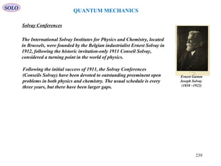
![•Quantity v
•t
•e
Symbol Value[7][8]
(SI units)
Relative Standard
Uncertainty
Bohr radius 5.291 772 1092(17) × 10−11
m 3.2 × 10⁻⁹
classical electron radius 2.817 940 3267(27) × 10−15
m 9.7 × 10⁻¹⁰
electron mass me 9.109 382 91(40) × 10−31
kg 4.4 × 10⁻⁸
Fermi coupling constant 1.166 364(5) × 10−5
GeV−2
4.3 × 10⁻⁶
fine-structure constant 7.297 352 5698(24) × 10−3
3.2 × 10⁻¹⁰
Hartree energy 4.359 744 34(19) × 10−18
J 4.4 × 10⁻⁸
proton mass mp 1.672 621 777(74) × 10−27
kg 4.4 × 10⁻⁸
quantum of circulation 3.636 947 5520(24) × 10−4
m² s−1
6.5 × 10⁻¹⁰
Rydberg constant 10 973 731.568 539(55) m−1
5.0 × 10⁻¹²
Thomson cross section 6.652 458 734(13) × 10−29
m² 1.9 × 10⁻⁹
weak mixing angle 0.2223(21) 9.5 × 10⁻³
Table of atomic and nuclear constants
SOLO
352](https://image.slidesharecdn.com/5-introductiontoquantummechanics-sololaptop-150813162751-lva1-app6891/85/5-introduction-to-quantum-mechanics-352-320.jpg)
![•Quantity v
•t
•e
Symbol Value[7][8]
(SI units)
Relative
Standard
Uncertainty
Atomic mass constant mu = 1 u 1.660 538 921(73) × 10−27
kg 4.4 × 10⁻⁸
Avogadro's number NA, L 6.022 141 29(27) × 1023
mol−1
4.4 × 10⁻⁸
Boltzmann constant K=kB=R/NA 1.380 6488(13) × 10−23
J·K−1
9.1 × 10⁻⁷
Faraday constant F=NA e 96 485.3365(21)C·mol−1
2.2 × 10⁻⁸
first radiation constant
c1 = 2 π h c2
3.741 771 53(17) × 10−16
W·m² 4.4 × 10⁻⁸
for spectral radiance c1L
1.191 042 869(53) × 10−16
W·m²
sr−1 4.4 × 10⁻⁸
Loschmidt constant
at =273.15 K and
=101.325 kPa
n0=NA/Vm 2.686 7805(24) × 1025
m−3
9.1 × 10⁻⁷
gas constant R 8.314 4621(75) J·K−1
·mol−1
9.1 × 10⁻⁷
molar Planck constant NAh 3.990 312 7176(28) × 10−10
J·s·mol−1 7.0 × 10⁻¹⁰
molar volume of an
ideal gas
at =273.15 K and =100
kPa
Vm=RT/p
2.271 0953(21) × 10−2
m³·mol−1
9.1 × 10⁻⁷
at =273.15 K and
=101.325 kPa
2.241 3968(20) × 10−2
m³·mol−1
9.1 × 10⁻⁷
Sackur-Tetrode
constant
at =1 K and =100 kPa −1.151 7078(23) 2.0 × 10⁻⁶
at =1 K and =101.325
kPa
−1.164 8708(23) 1.9 × 10⁻⁶
second radiation constant c2=hc/k 1.438 7770(13) × 10−2
m·K 9.1 × 10⁻⁷
Stefan–Boltzmann constant 5.670 373(21) × 10−8
W·m−2
·K−4
3.6 × 10⁻⁶
Wien displacement law constant B=hck-1
/4.965 114 231... 2.897 7721(26) × 10−3
m·K 9.1 × 10⁻⁷
Table of physico-chemical constantsSOLO
353](https://image.slidesharecdn.com/5-introductiontoquantummechanics-sololaptop-150813162751-lva1-app6891/85/5-introduction-to-quantum-mechanics-353-320.jpg)
![Name vte Dimension Expression Value[11]
(SI units)
Planck length
Length (L)
1.616 199(97) × 10 −35
m[12]
Planck mass Mass (M) 2.176 51(13) × 10 −8
kg[13]
Planck time Time (T) 5.391 06(32) × 10 −44
s[14]
Planck charge Electric charge (Q)
1.875 545 956(41) × 10 −18
C
[15][16][17]
Planck temperature Temperature (Θ) 1.416 833(85) × 10 32
K[18]
SOLO
354](https://image.slidesharecdn.com/5-introductiontoquantummechanics-sololaptop-150813162751-lva1-app6891/85/5-introduction-to-quantum-mechanics-354-320.jpg)
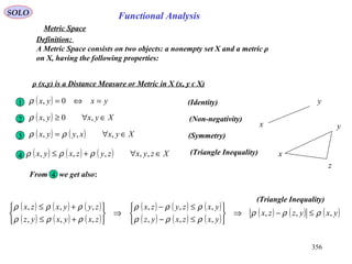
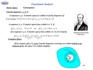
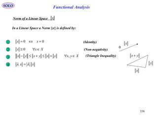
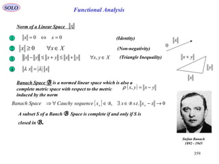
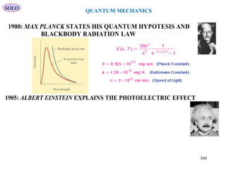
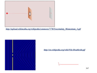
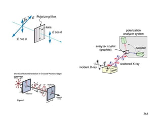
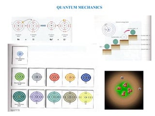
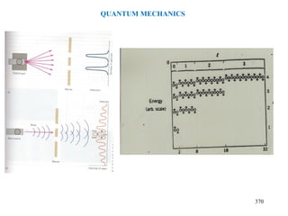
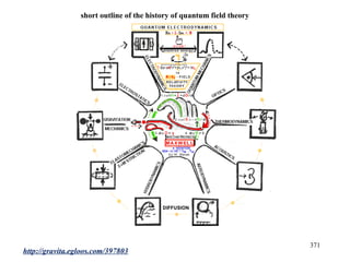
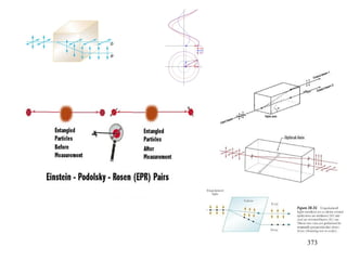
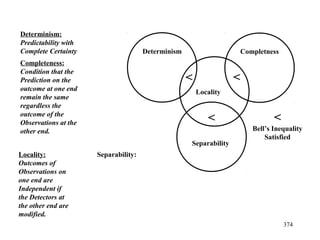
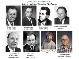
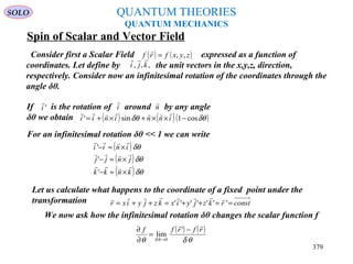
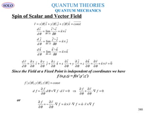
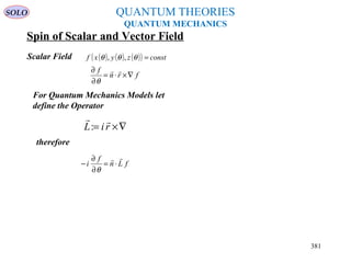
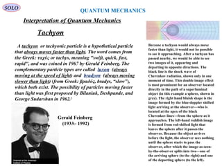
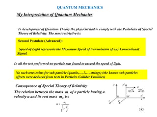
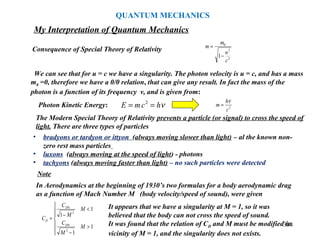
![The theoretical physics resolution of this paradox is to
assume the existence of virtual particles which pop out
of the vacuum and wander around for an undefined
time and then pop back – thus giving the vacuum an
average zero point energy, but without disturbing the
real world too much.
SOLO
385
QUANTUM MECHANICS
In quantum physics, a quantum vacuum fluctuation
(or quantum fluctuation or vacuum fluctuation) is the
temporary change in the amount of energy in a point
in space,[1]
arising from Werner Heisenberg's
uncertainty principle.
The so called “stable particles” (life time greater than Planck Time = 10-43
sec ) interacts
continuously with the vacuum sub-particles (quarks,…,?,…,strings) in such a way that the
“stable particles”:
-retain their internal structure (possible by exchanging quarks) and acts as a “stable” wave that
doesn’t dissipate, because of the internal gluons that binds the internal quarks.
-Those interactions may happen at times shorter than the Planck Time, therefore are not
necessarily observable.
-transfer their internal “DNA” to the vacuum sub-particles.
-Those sub-particle, of zero mass, will spread this information, by traveling with speeds that
“cross the speed of light” in contradiction to Einstein Postulate.
-Those are the non-local Pilot-Waves of de Broglie-Bohm Theory.
My Interpretation of Quantum Mechanics](https://image.slidesharecdn.com/5-introductiontoquantummechanics-sololaptop-150813162751-lva1-app6891/85/5-introduction-to-quantum-mechanics-385-320.jpg)

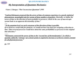
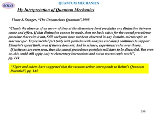
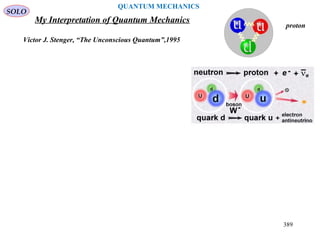
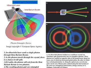

The document is a comprehensive overview of quantum mechanics, spanning its historical development, fundamental principles, and key theories. It discusses significant milestones in the field, including the discovery of the electron, the development of the Schrödinger equation, and interpretations of quantum mechanics like the Copenhagen interpretation. The author expresses a desire to share their findings and invites feedback on their presentation.


