Downloaded 90 times
![Matrix Multiplication
For two matrices A (of size l×m) and B (of size m×n), the product of AB
is defined by
where i = 1, 2, ..., l; j = 1, 2, ..., n.
Transpose of a Matrix
If A = [aij], then the transpose of A is](https://image.slidesharecdn.com/introductionfea-170628050705/75/Introduction-fea-17-2048.jpg)


This lecture provides an introduction to finite element analysis (FEA). It discusses the basic concepts of FEA, including dividing a complex object into simple finite elements and using polynomial terms to describe field quantities within each element. The lecture covers the history and applications of FEA, as well as the basic procedure, which involves meshing a structure into elements, describing element behavior, assembling elements at nodes, solving the system of equations, and calculating results. It also reviews matrix algebra concepts needed for FEA. Finally, it presents the simple example of a spring element and spring system to demonstrate the finite element modeling process.
Overview of the course on FEA from the School of Mechanical Engineering.
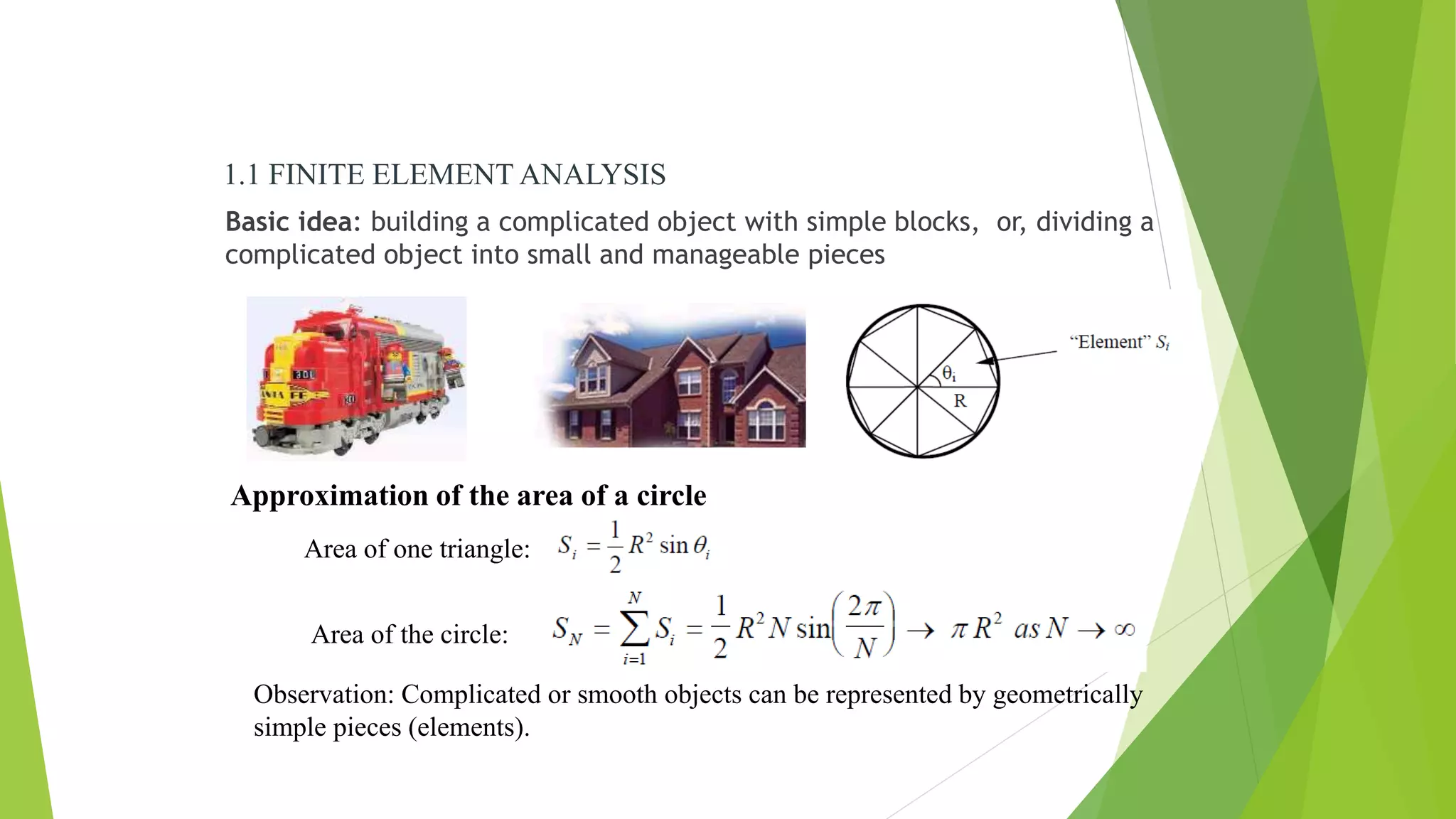
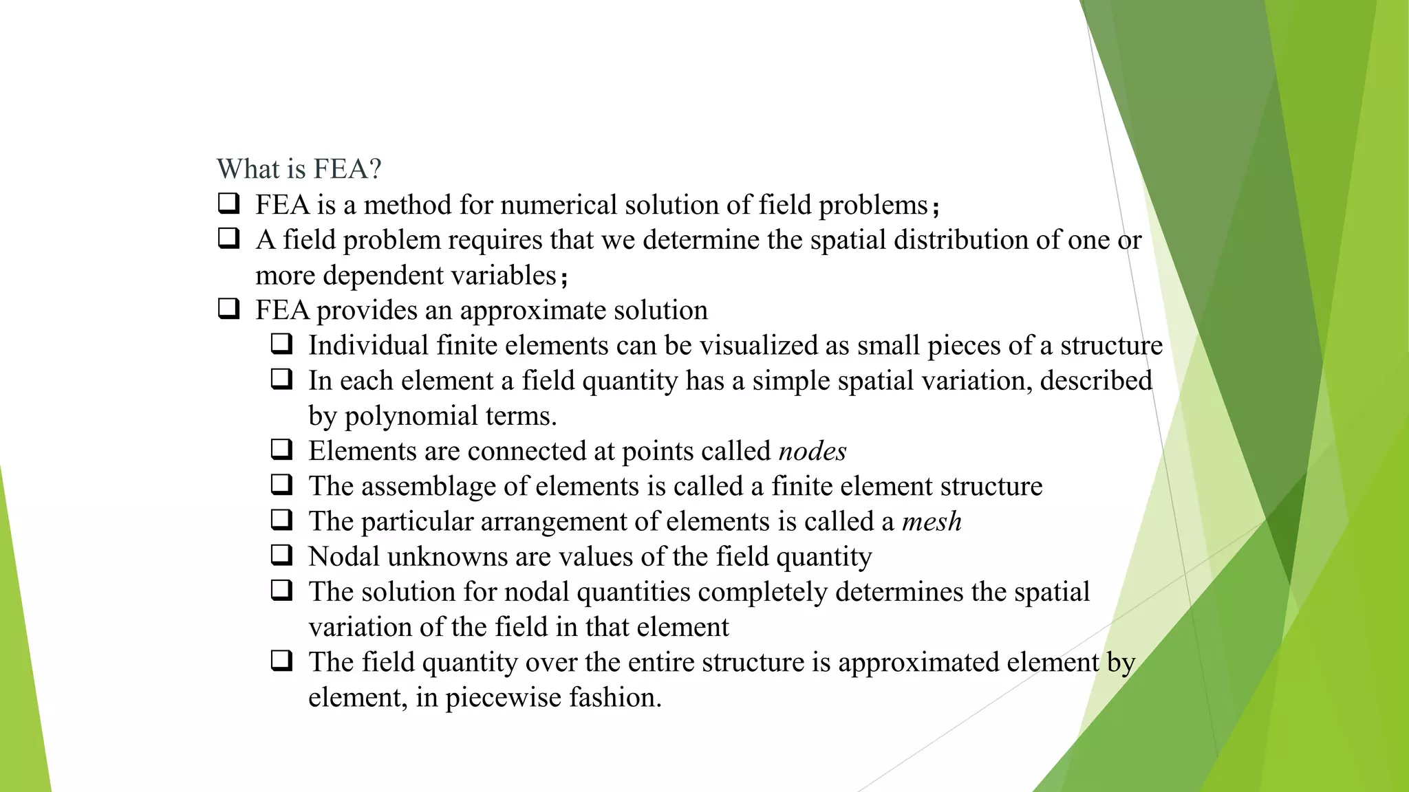
Basic concepts of FEA, approximating complex shapes with simple elements, and the importance of geometric representation.
FEA as a numerical method for field problems, involving element connections at nodes and mesh formation.
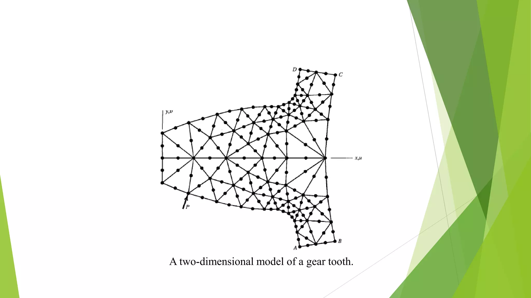
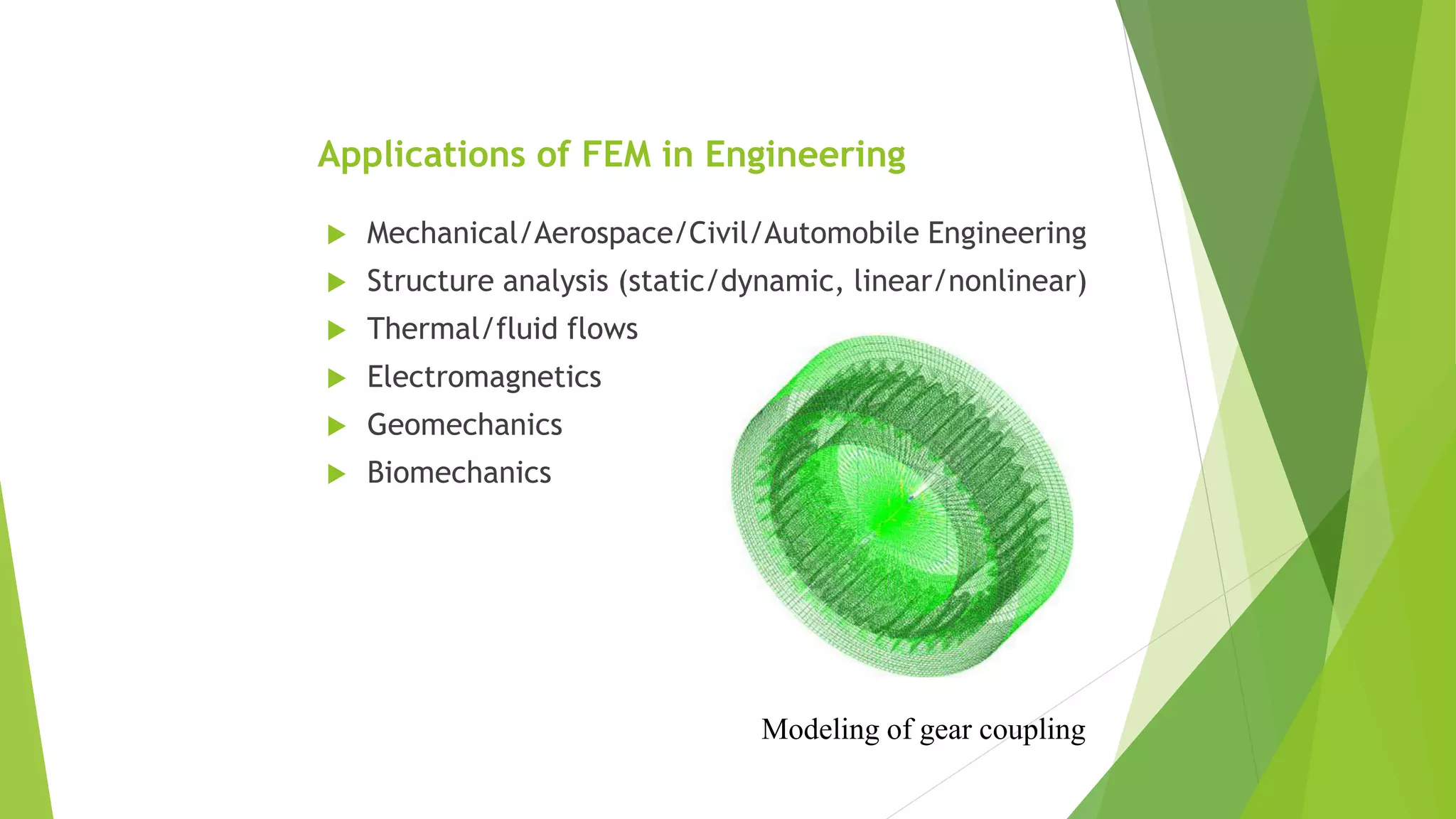
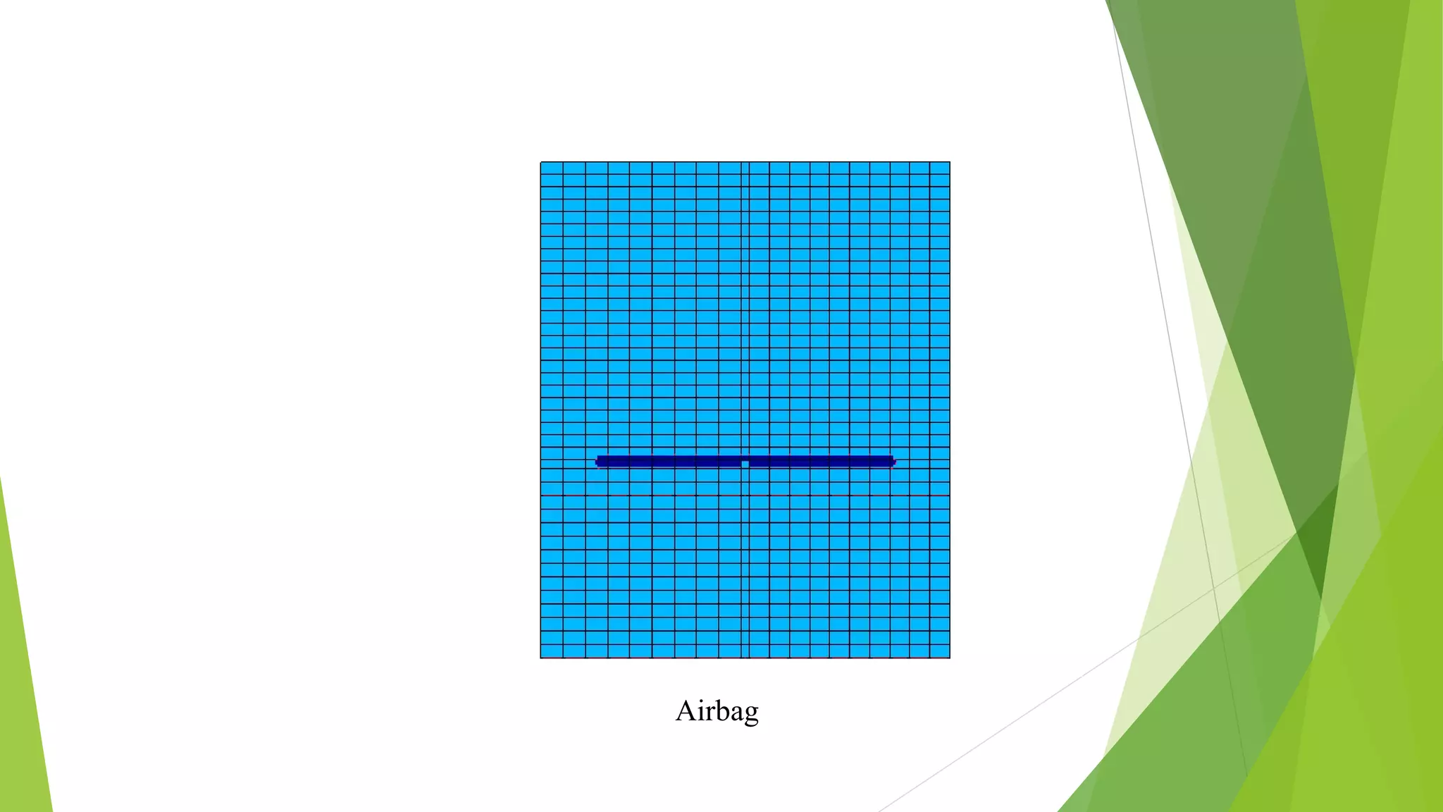
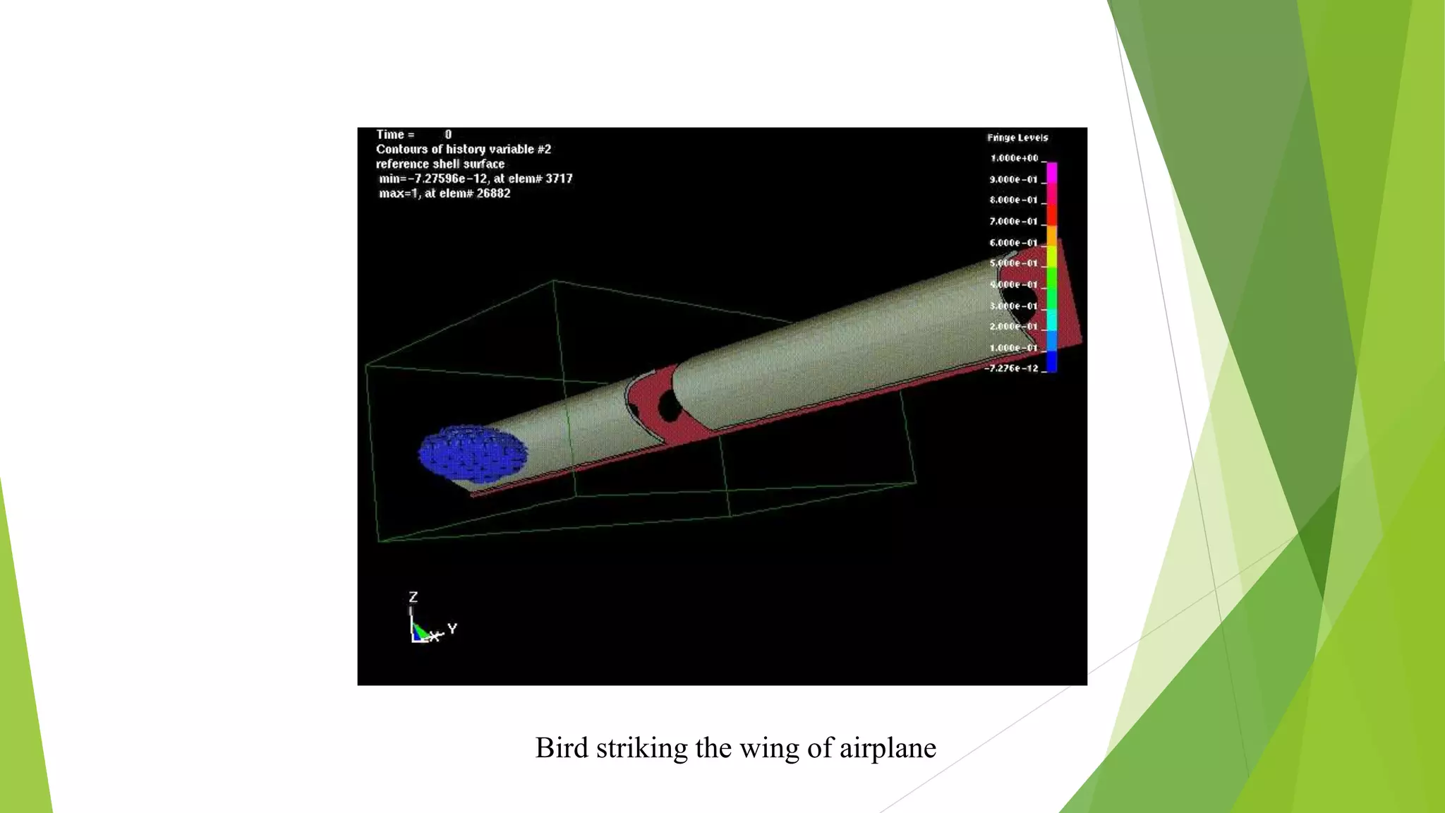
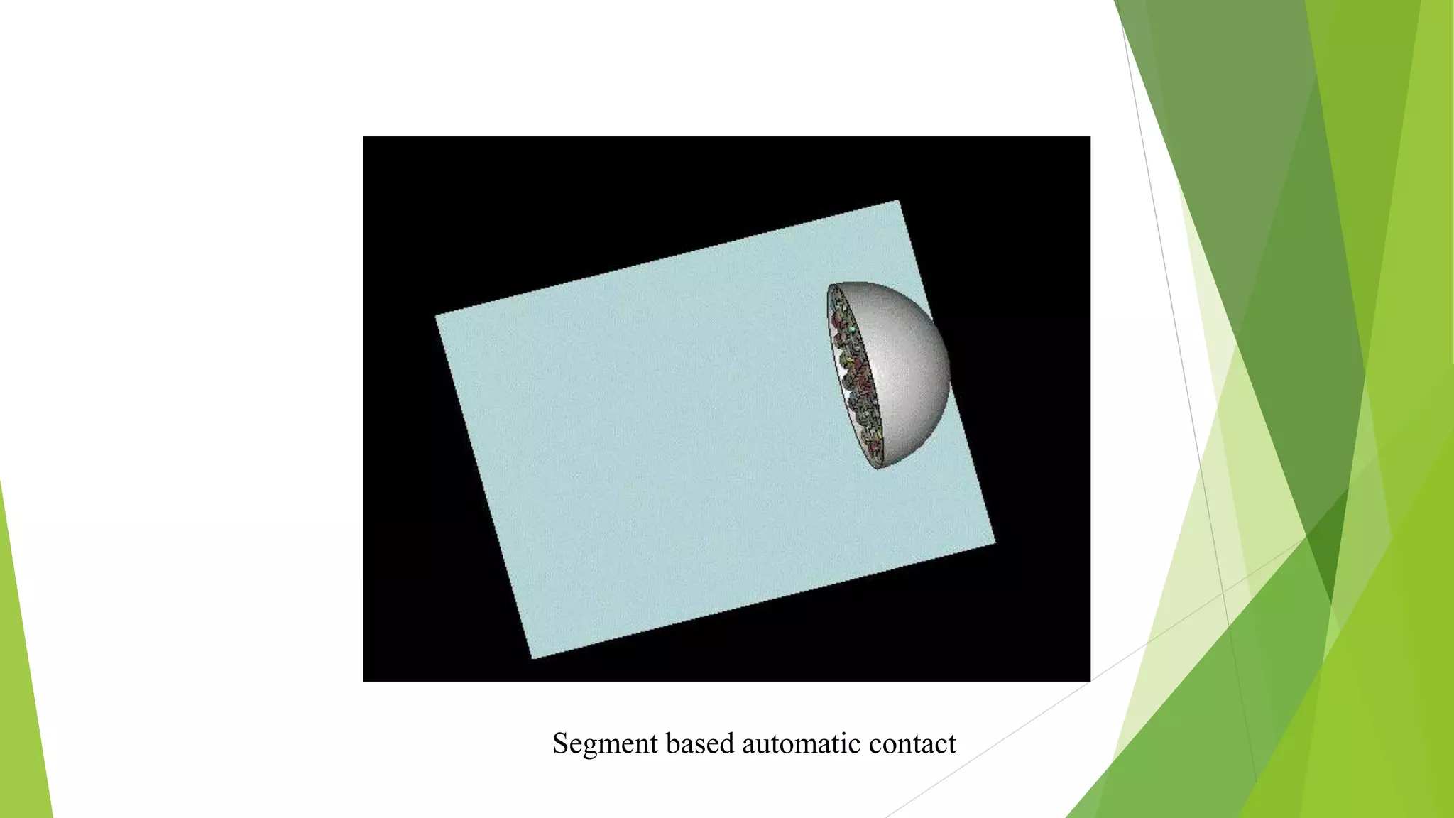
Various engineering applications of FEA including mechanical, aerospace, civil, automobile, and more.
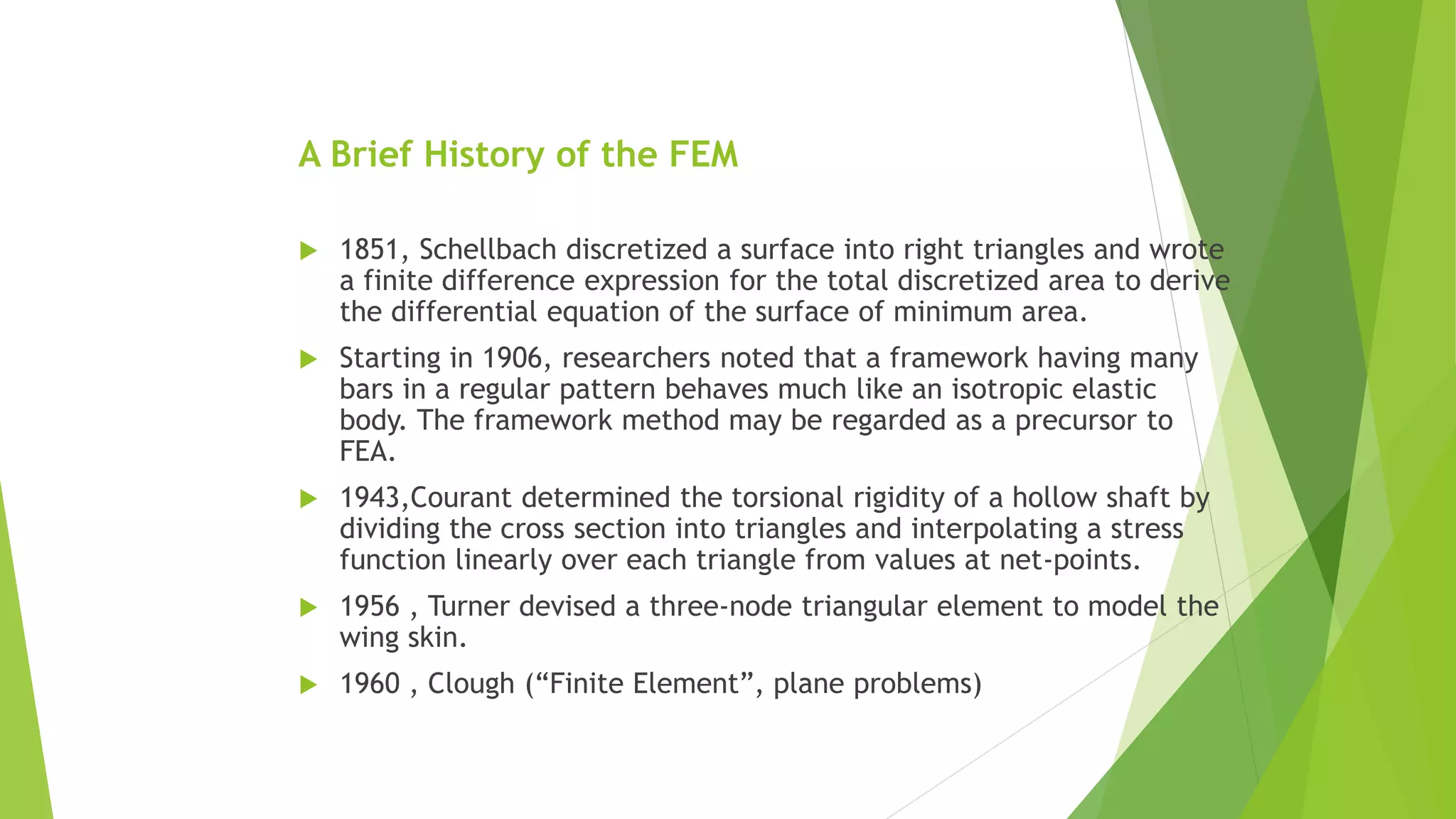
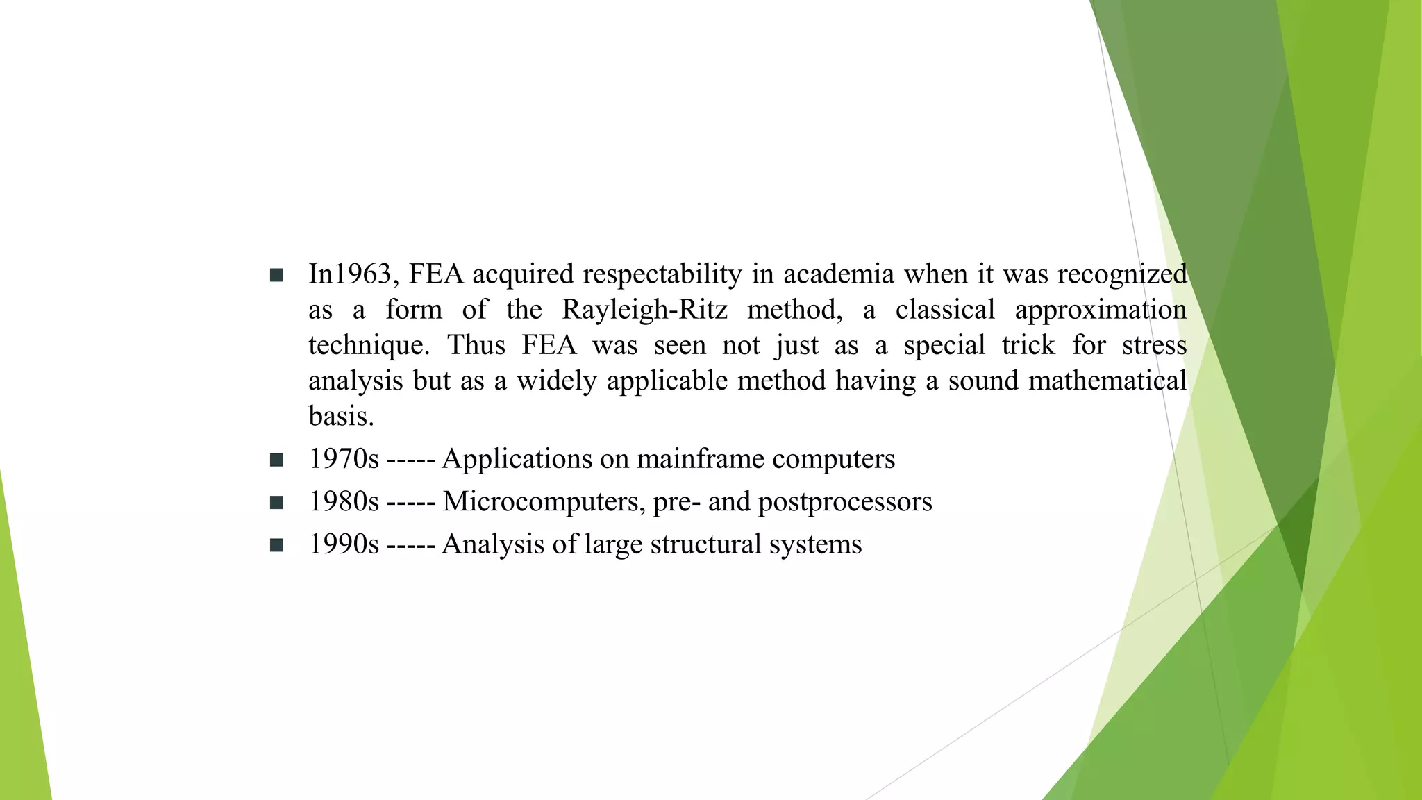
Chronological development of FEM from early discretization methods to modern applications and respectability in academia.
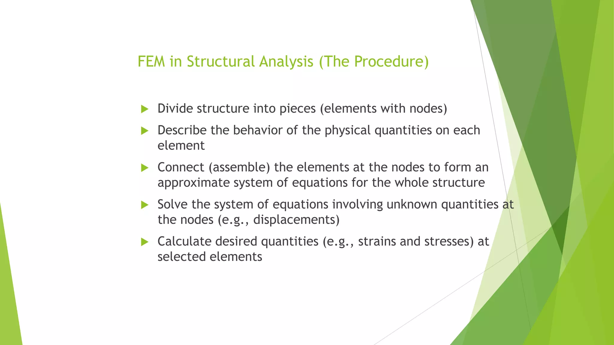
The step-by-step procedure for FEM in structural analysis, from dividing structures to calculating desired quantities.
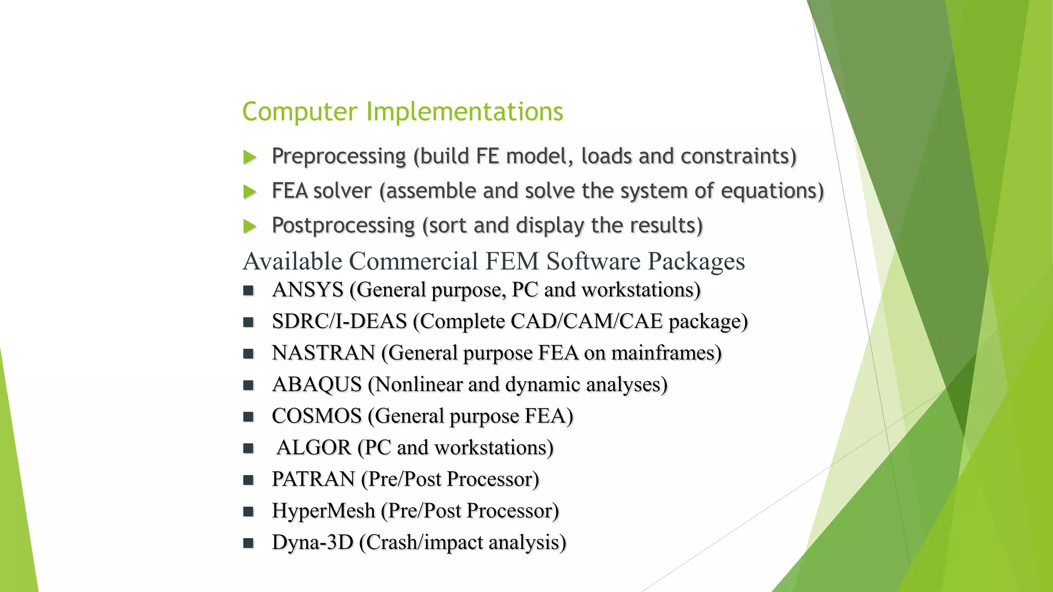
Overview of the preprocessing, solvers, and postprocessing stages in FEA, along with available software packages.
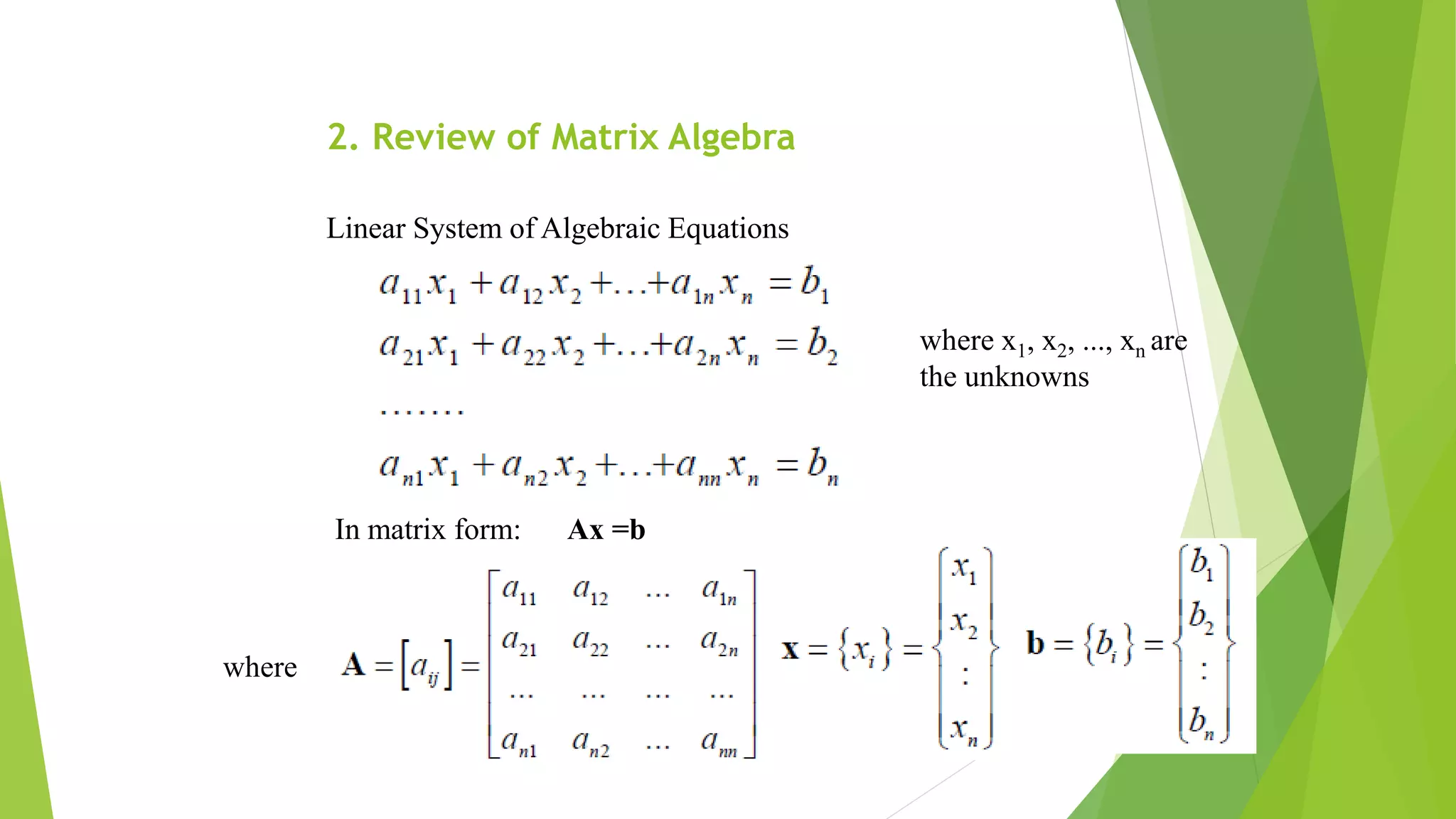
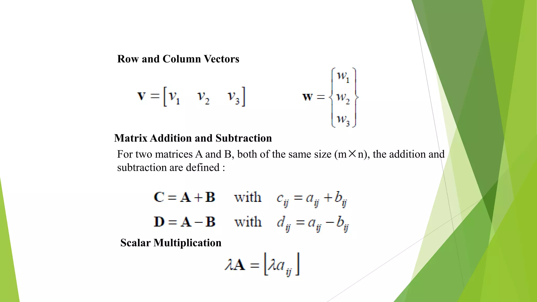
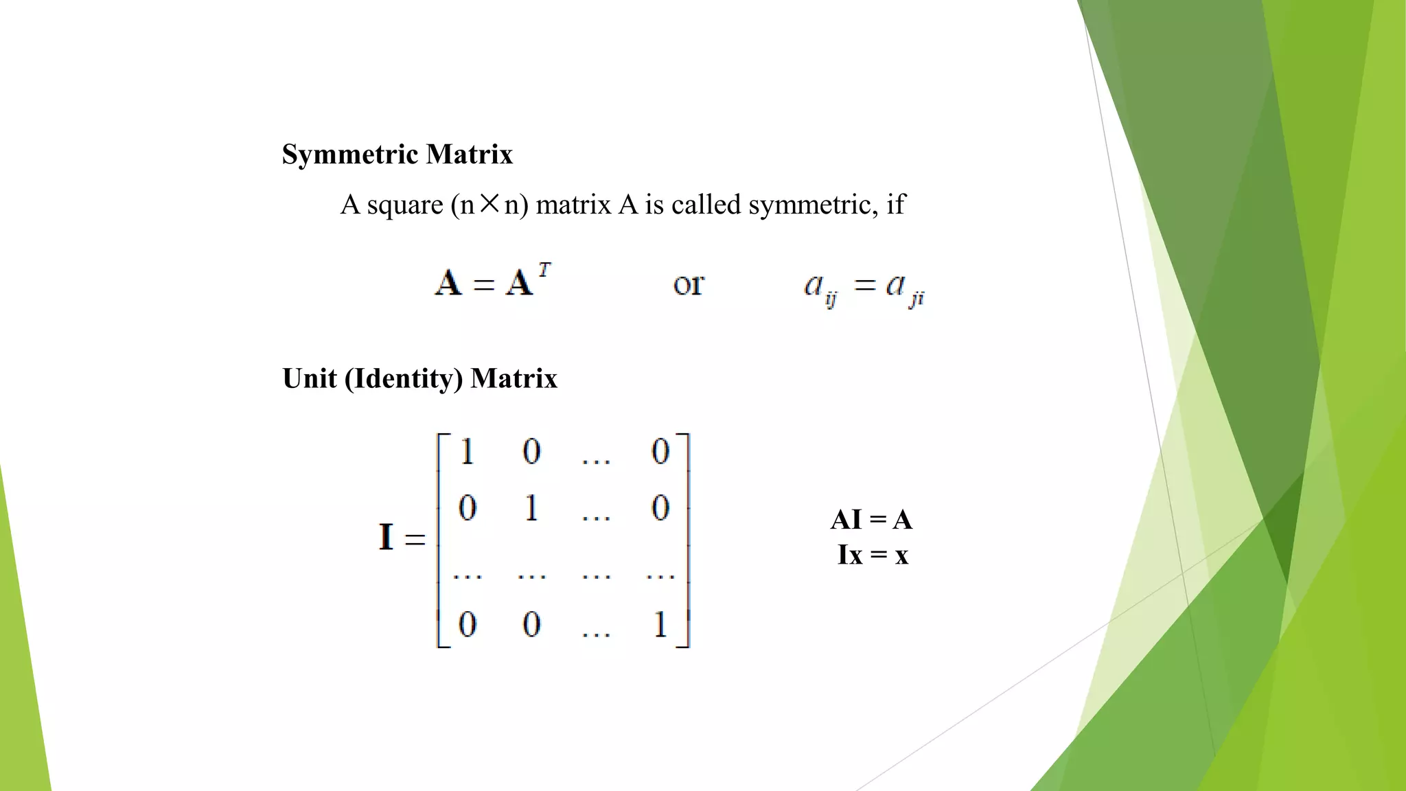
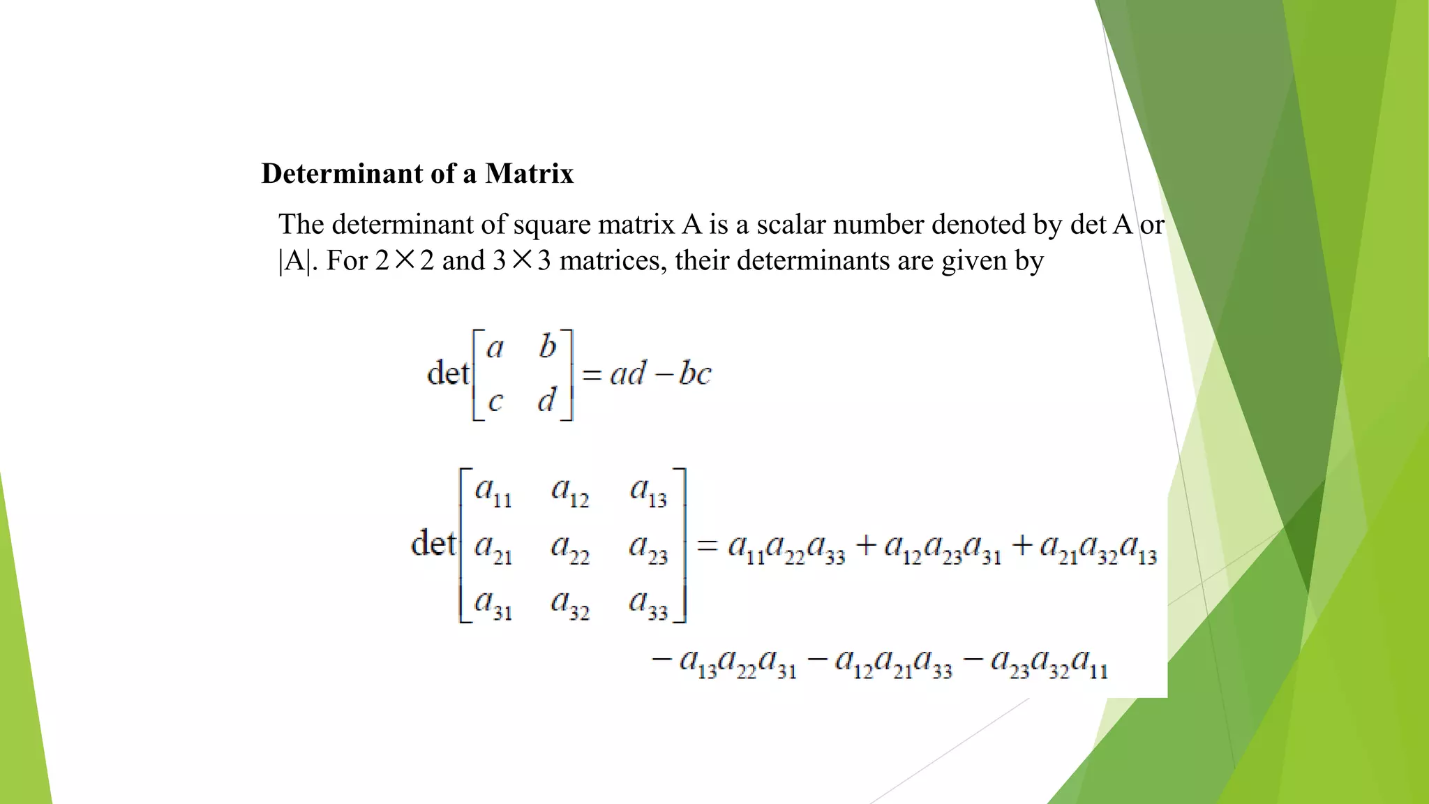
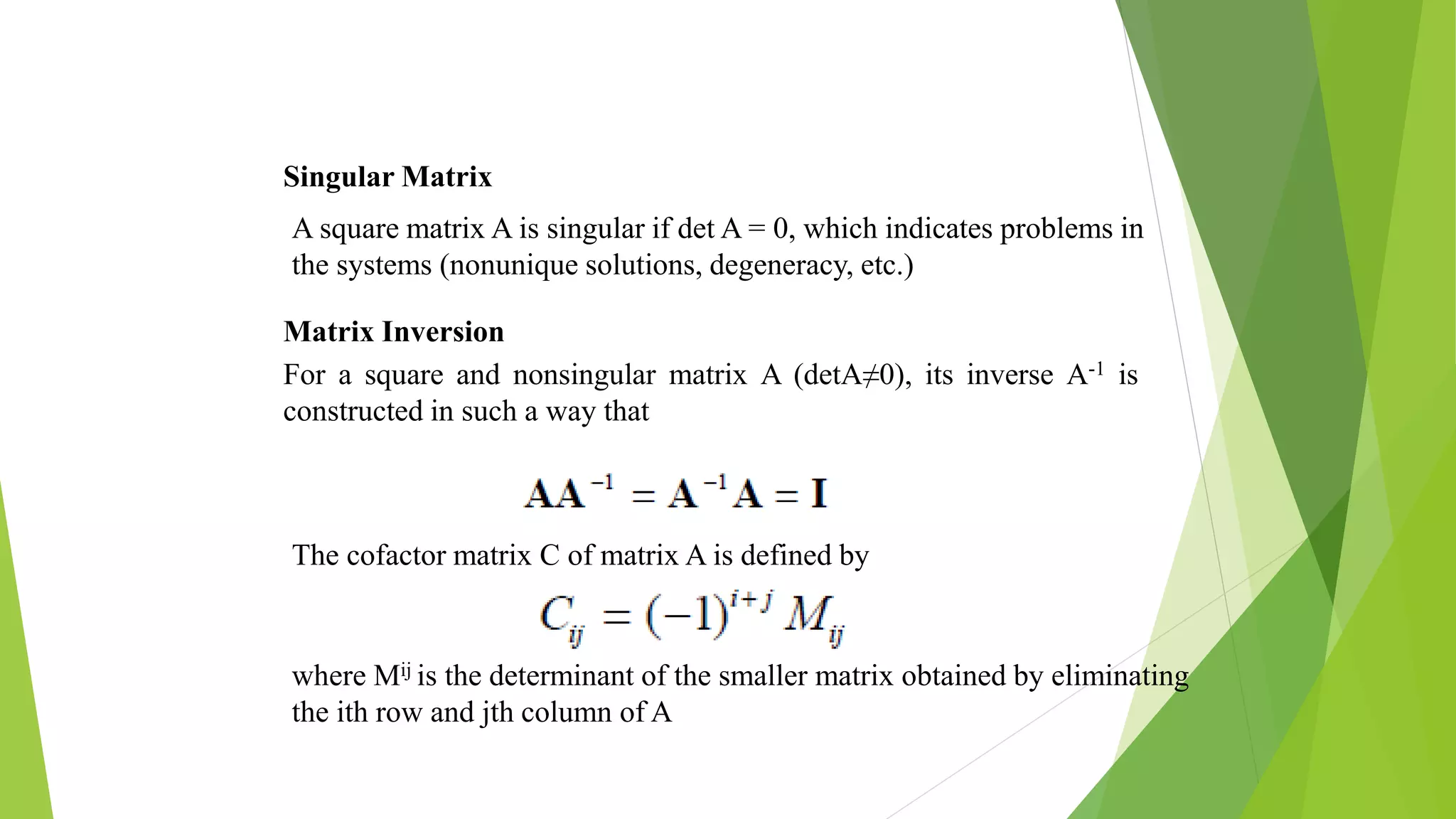
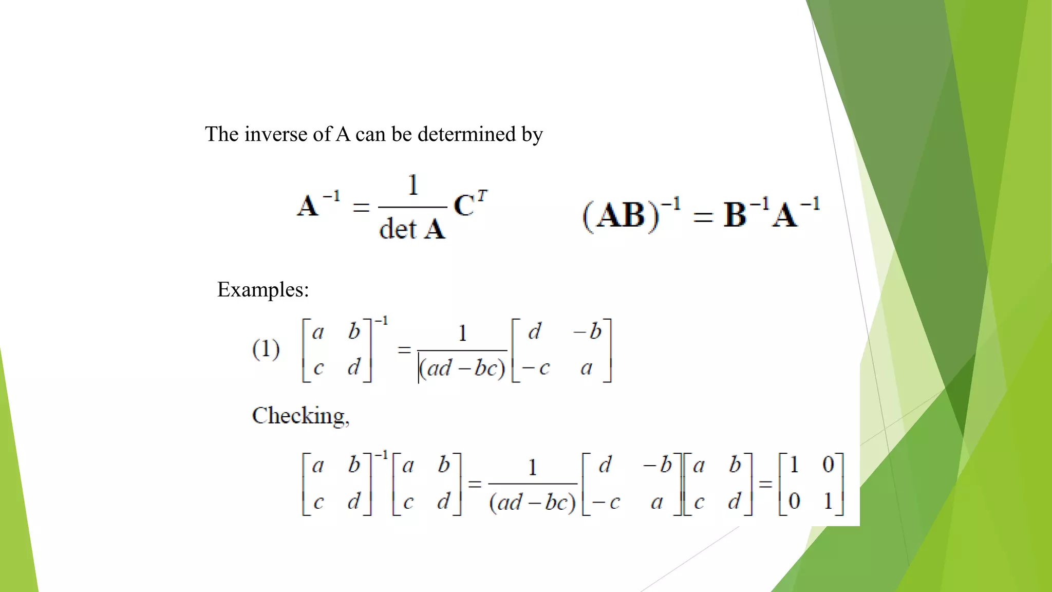
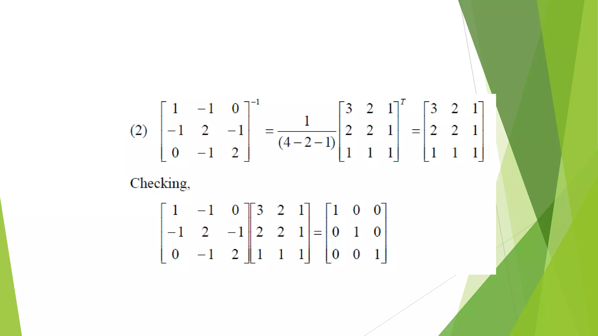
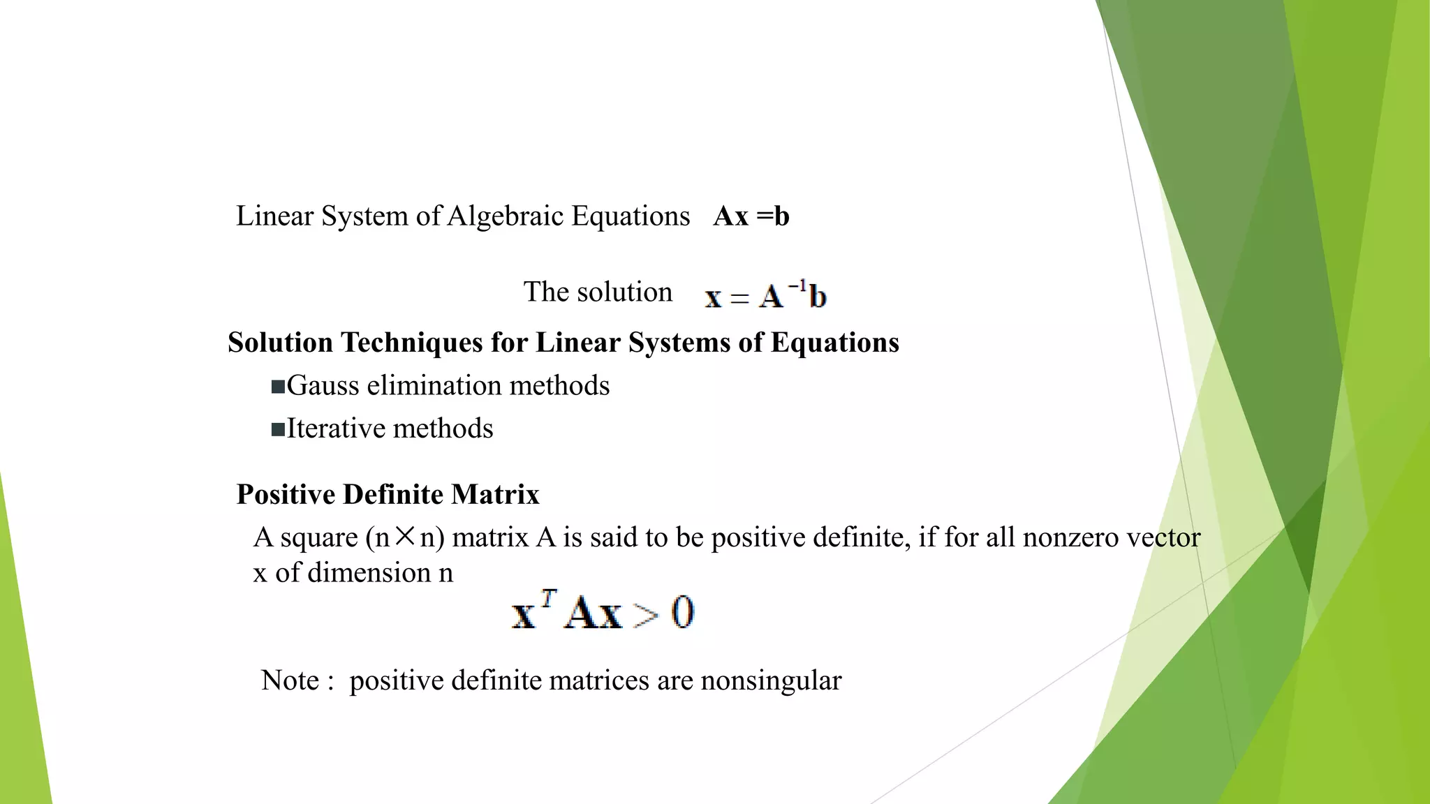
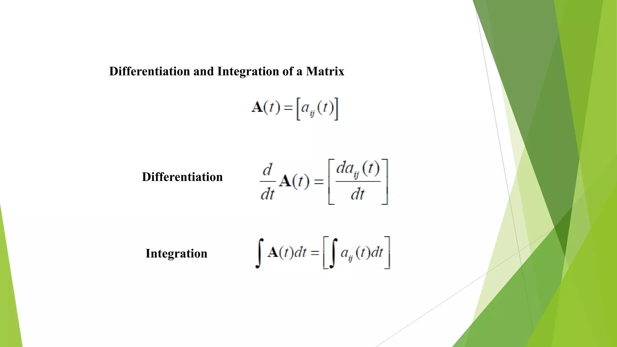
Key concepts in matrix algebra relevant to FEA, including systems of equations, matrix operations, and properties.
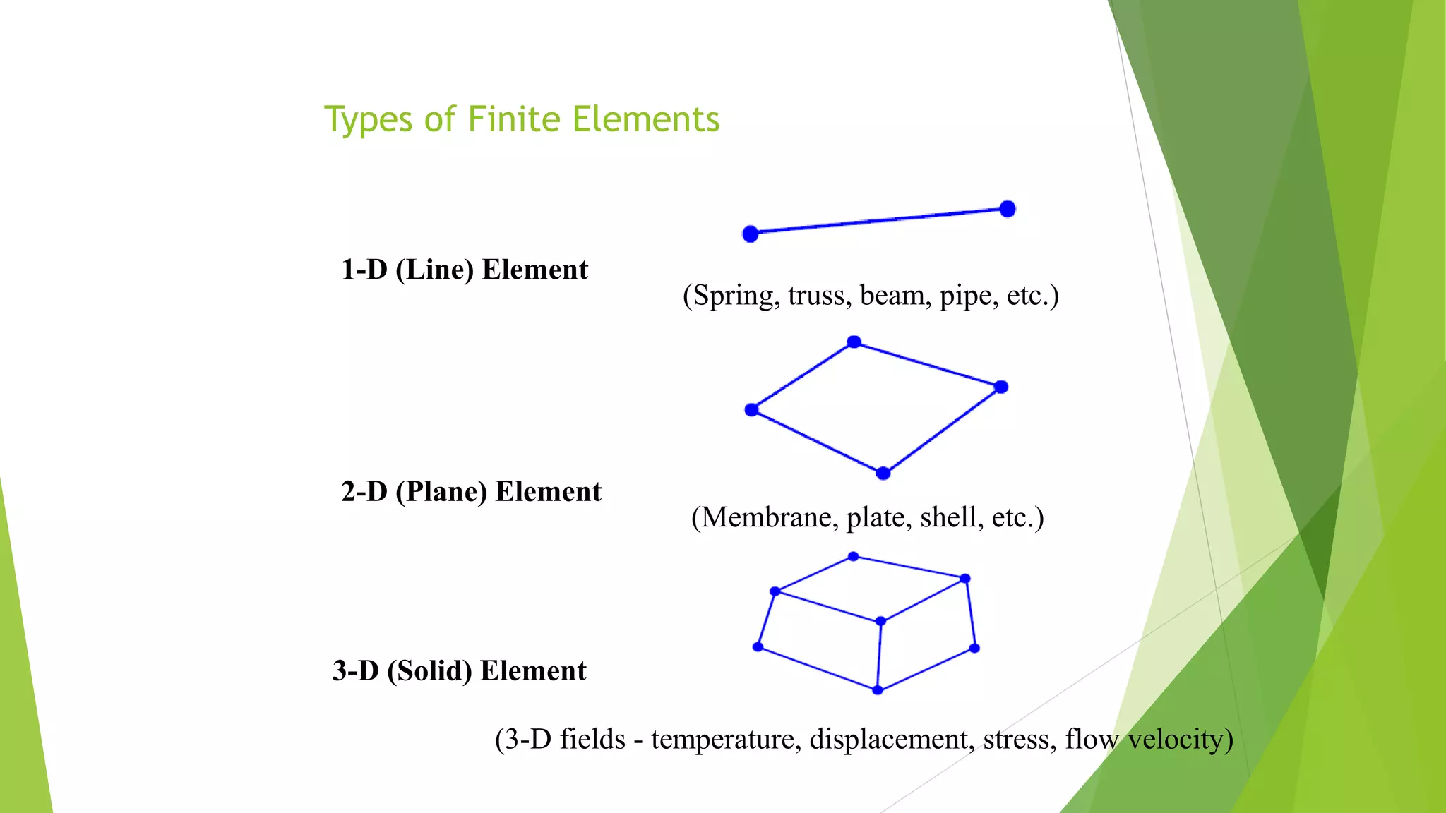
Introduction to different types of finite elements: 1D, 2D, and 3D elements used in various applications.
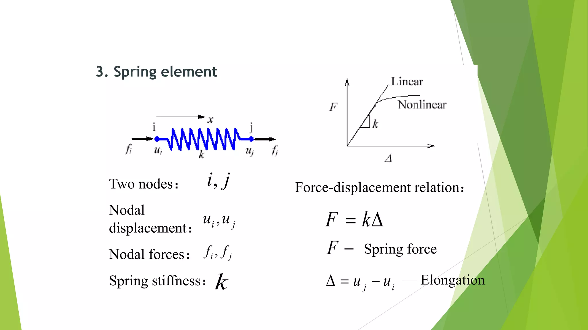
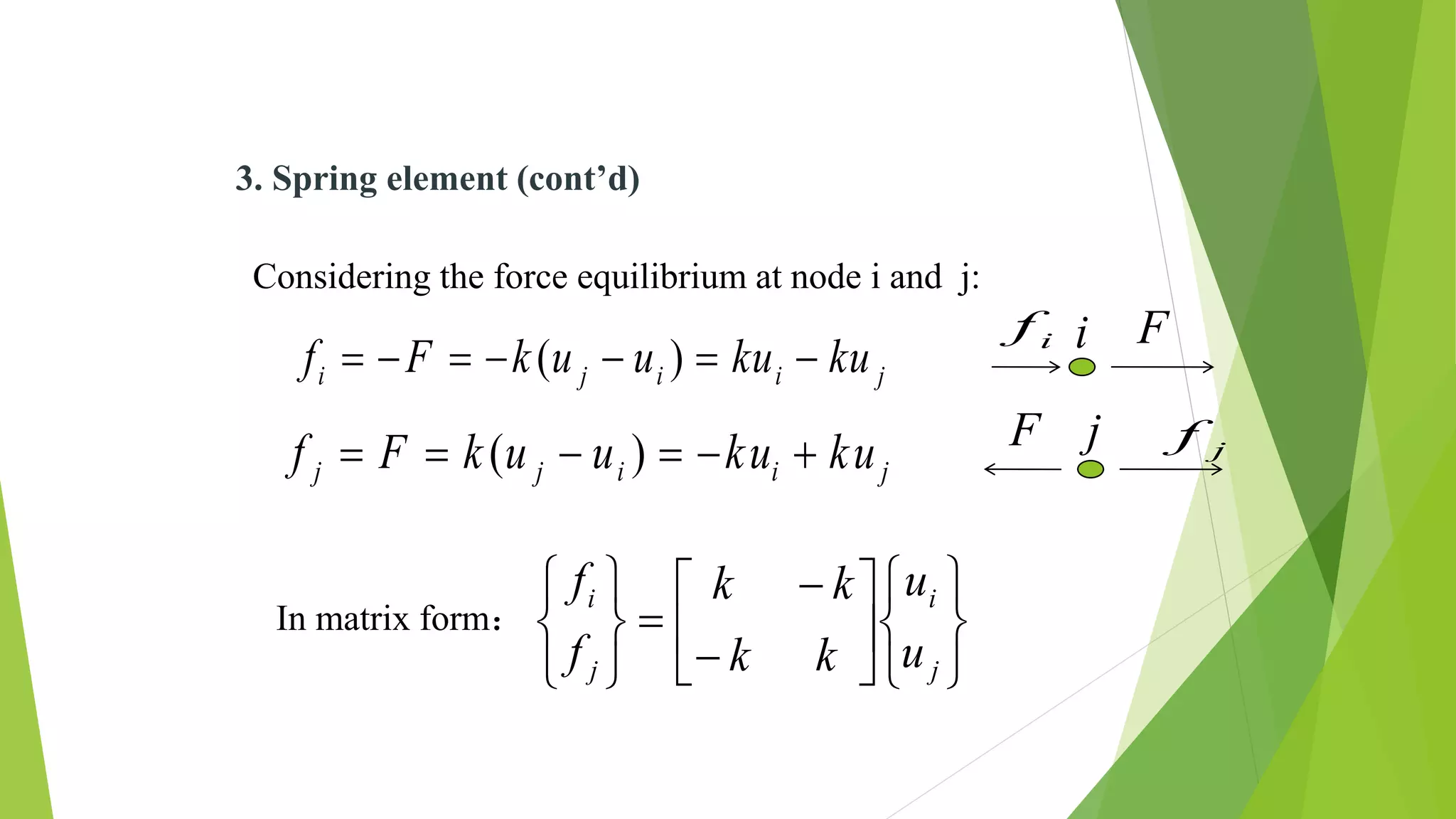
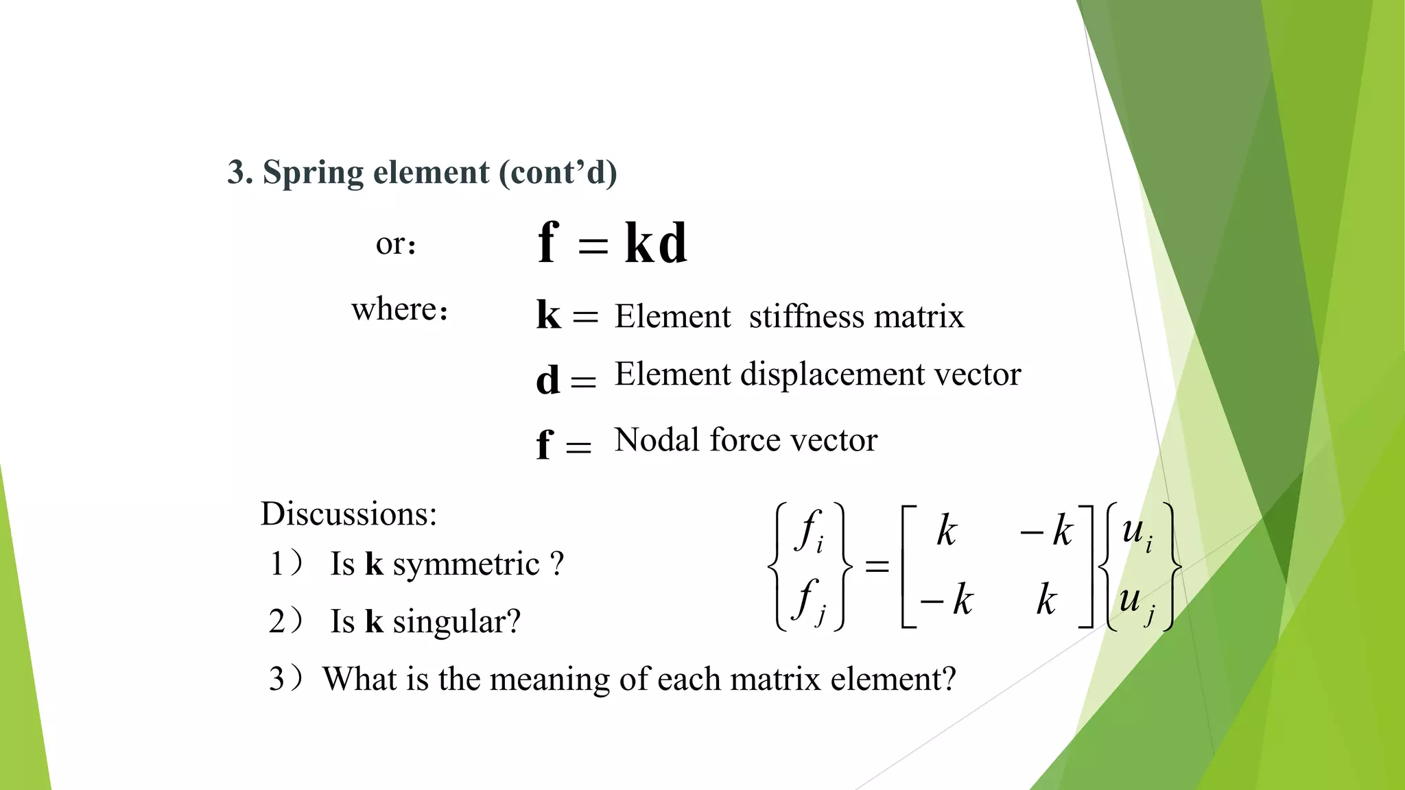
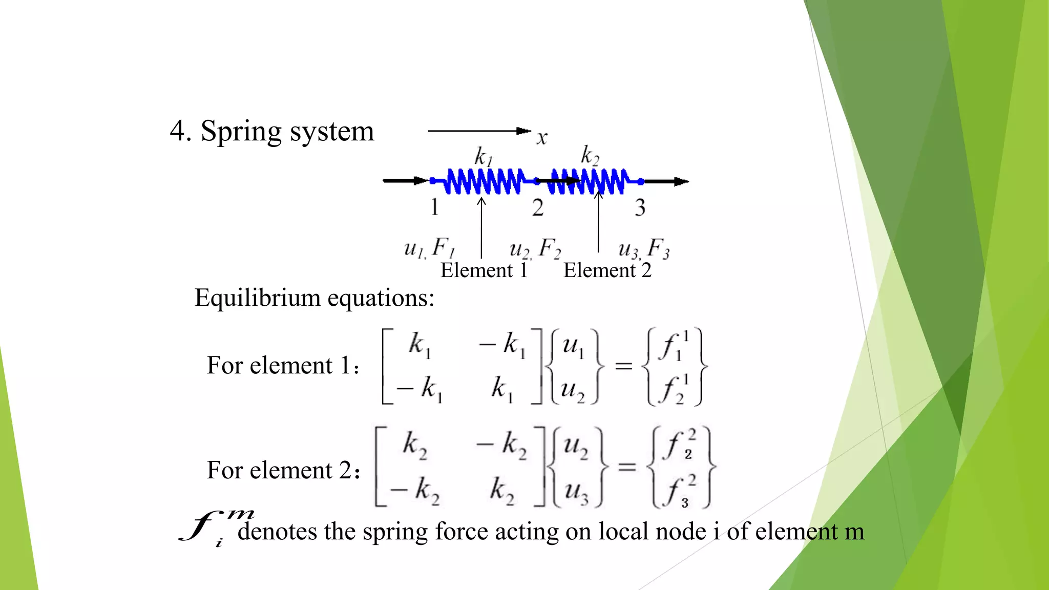
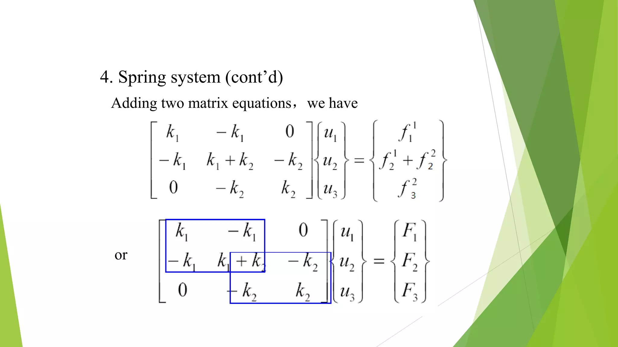
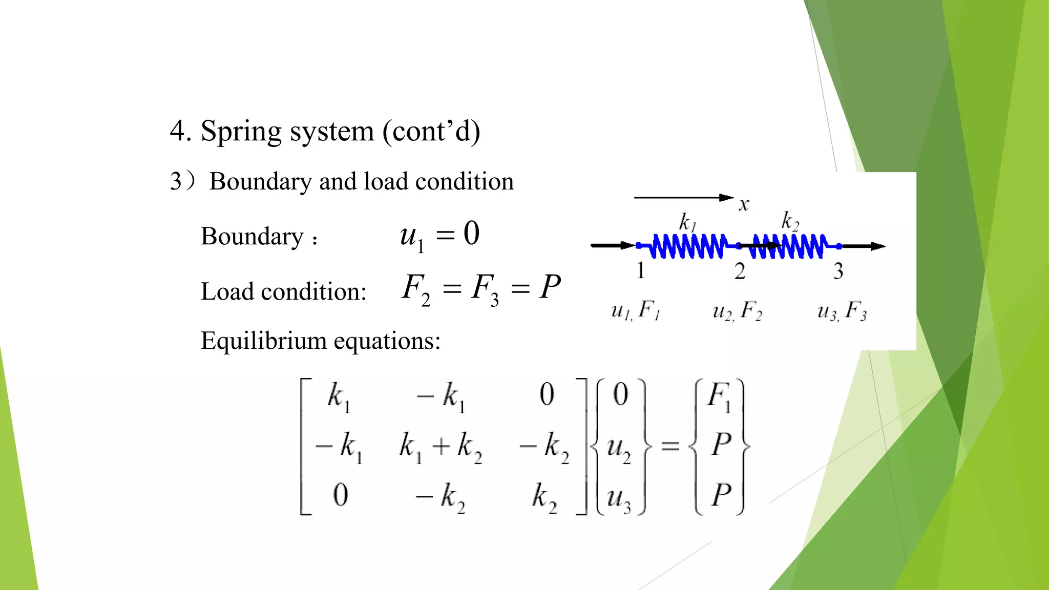
Detailed explanation of spring elements in FEA, including force-displacement relationships and equilibrium equations.
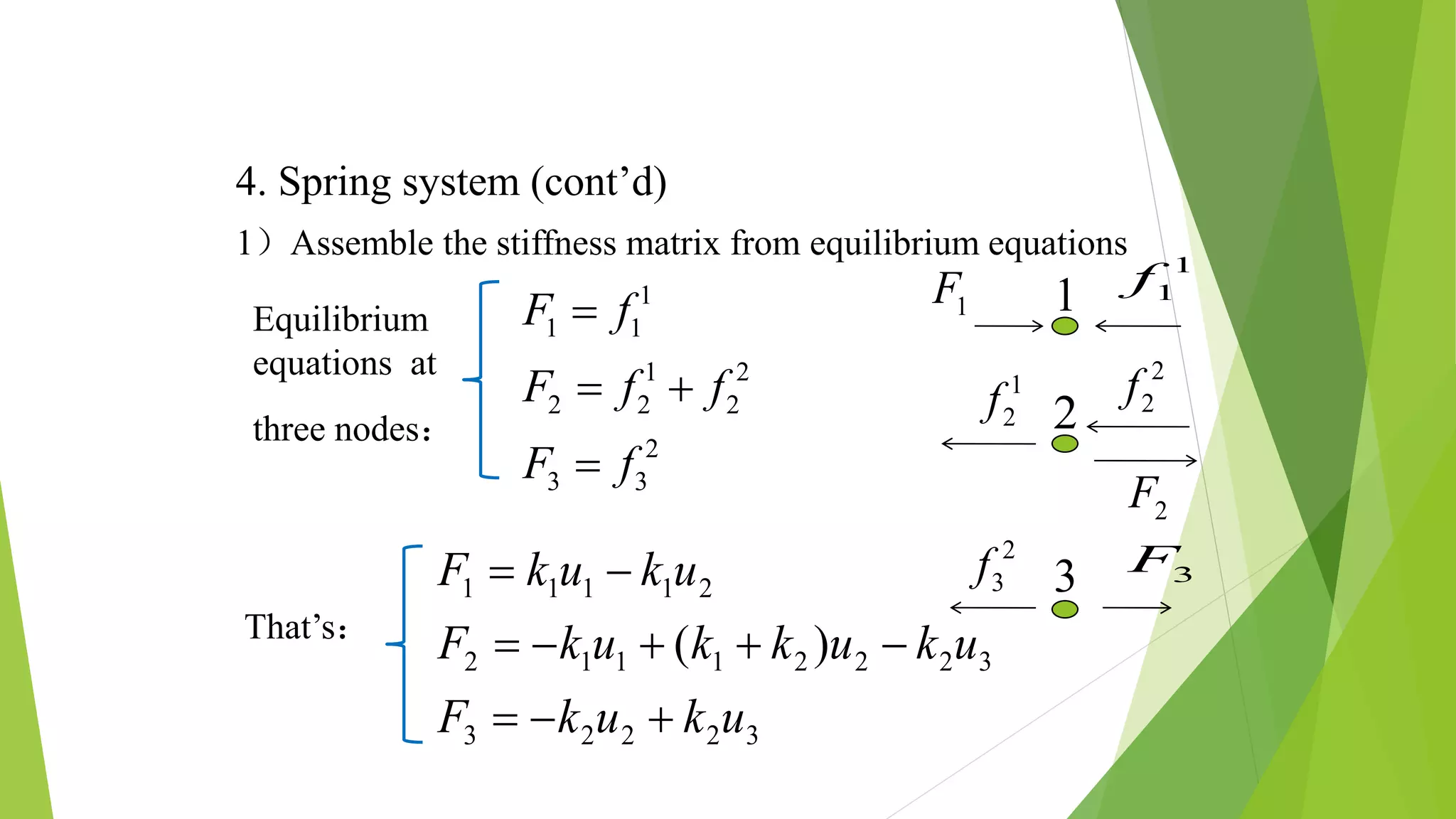
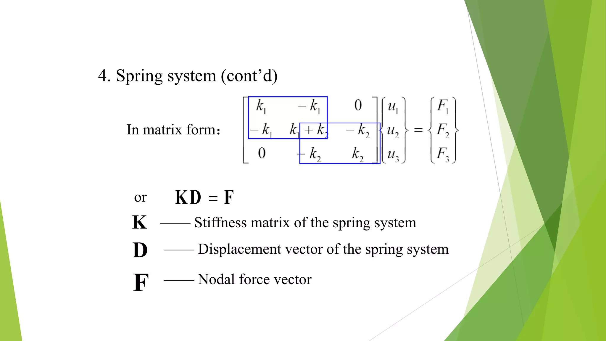
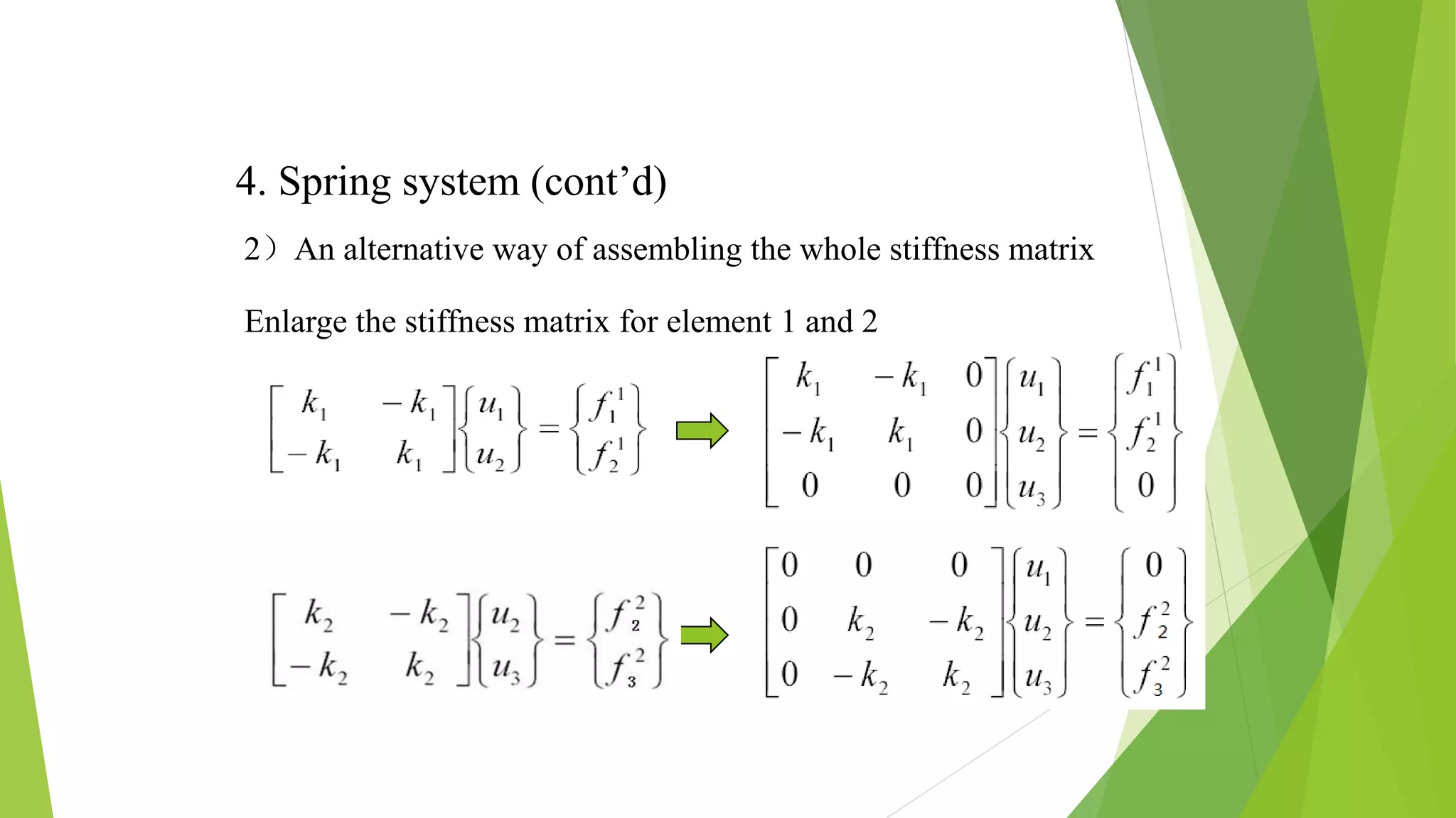
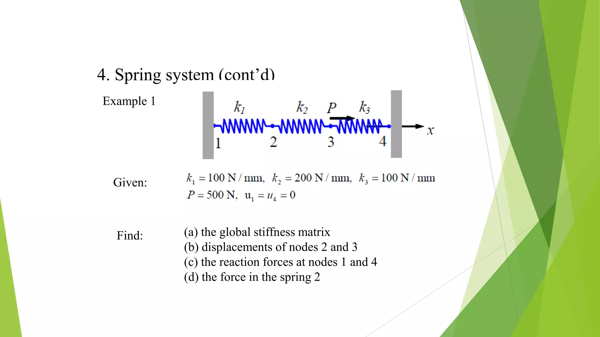
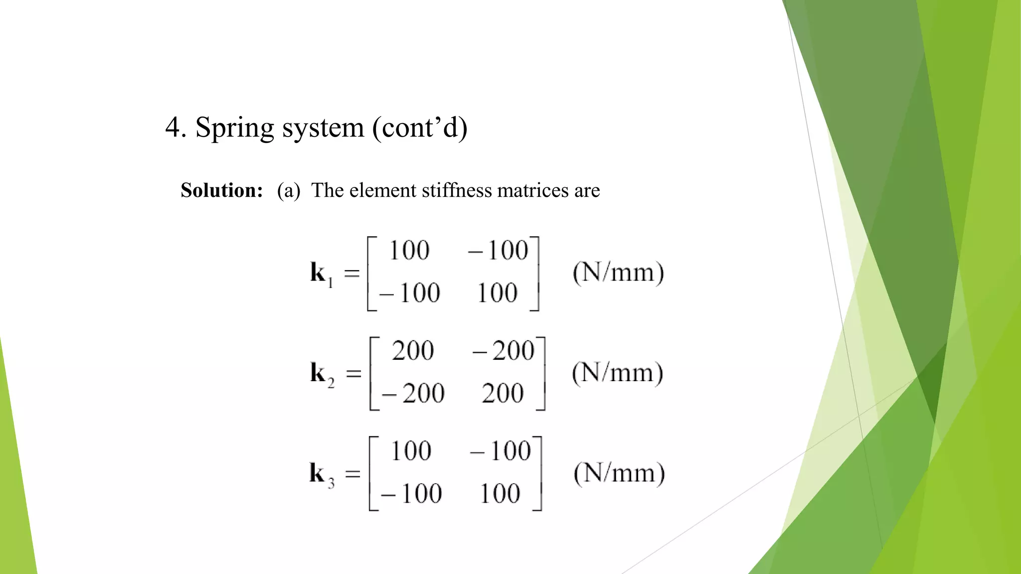
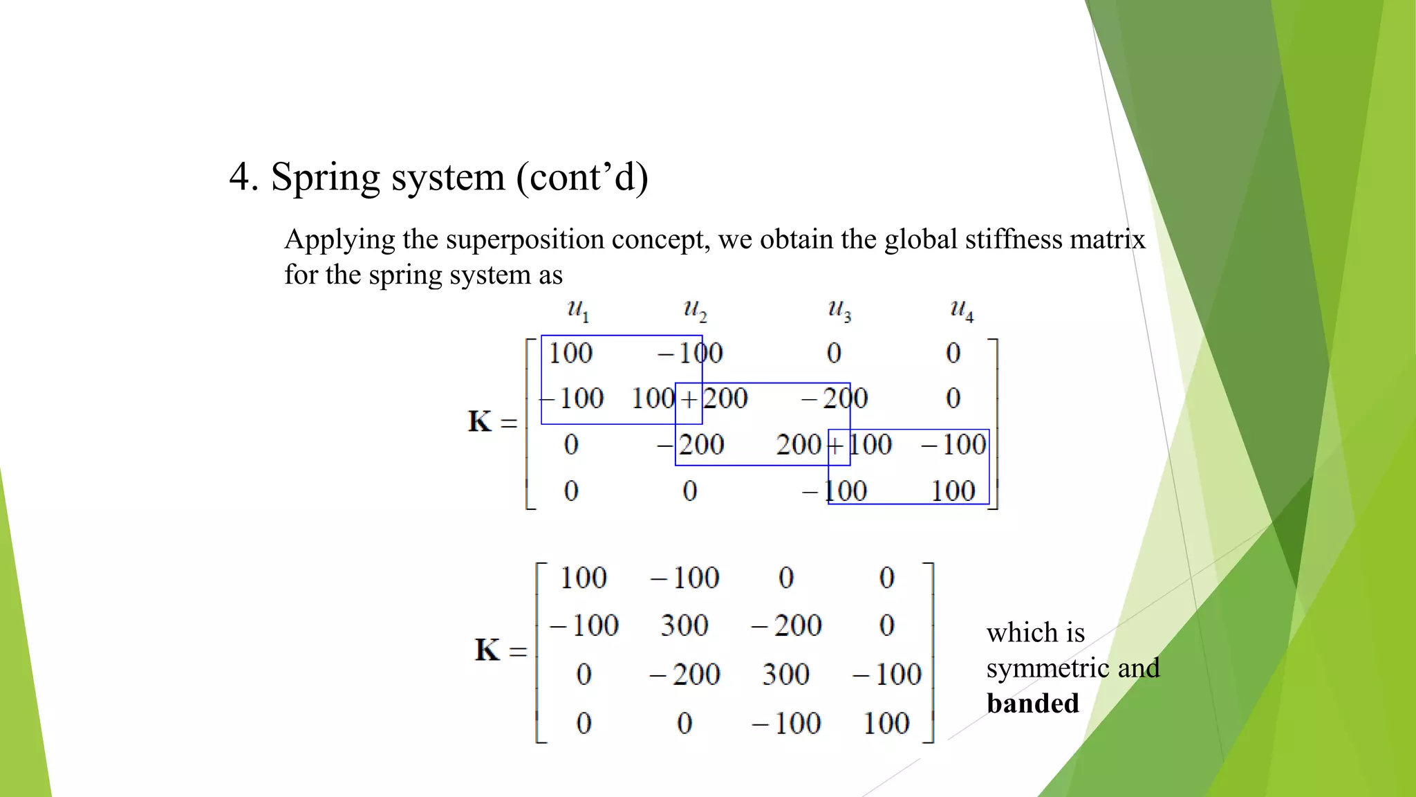
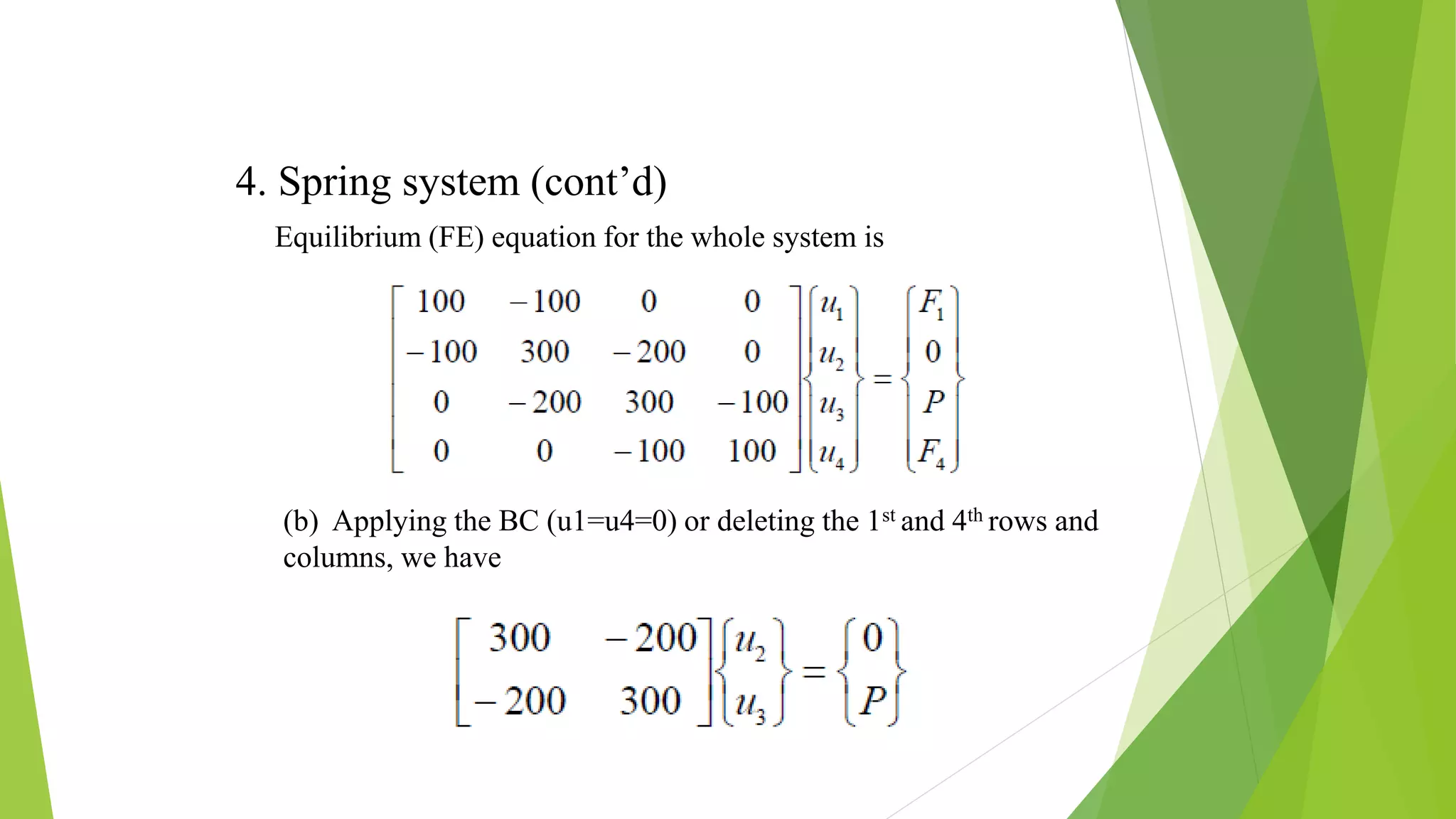
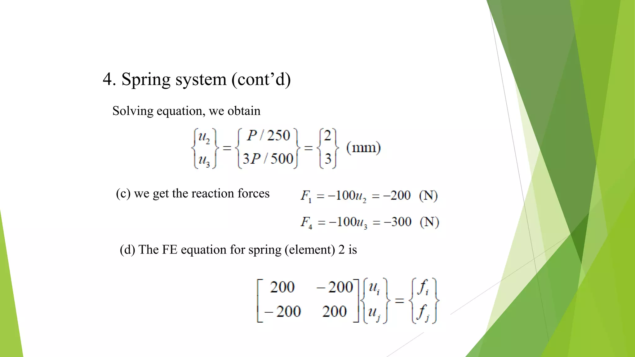
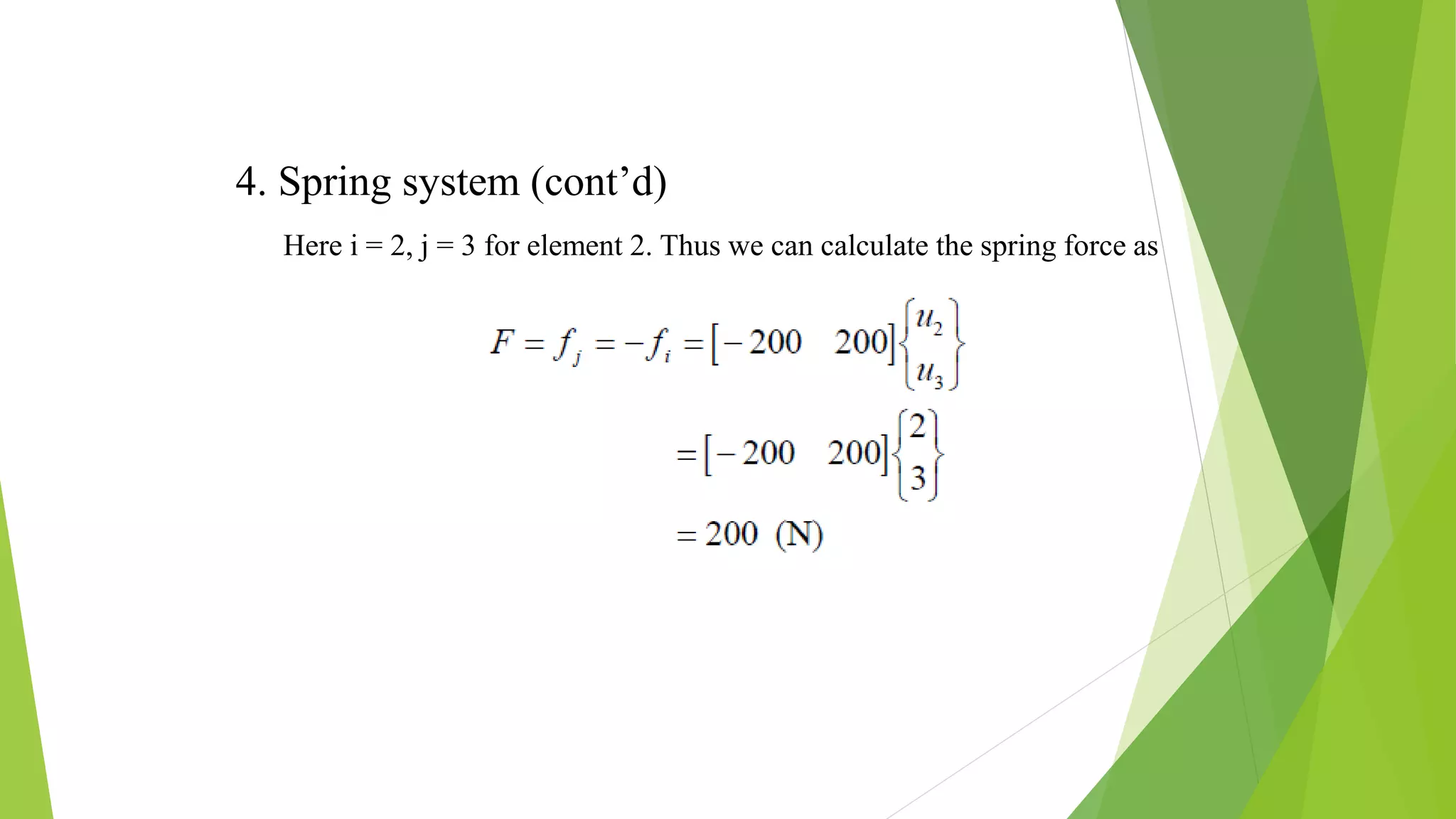
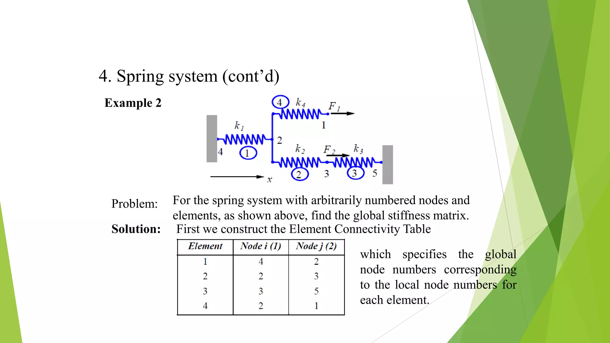
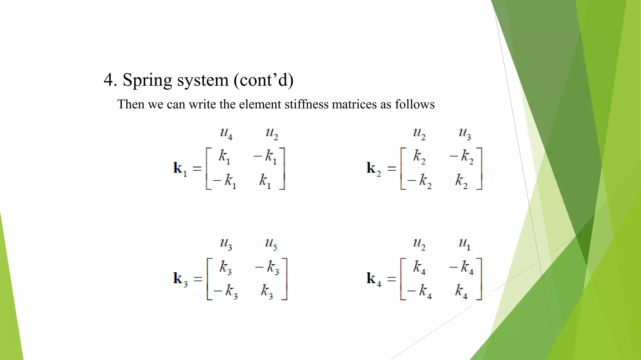
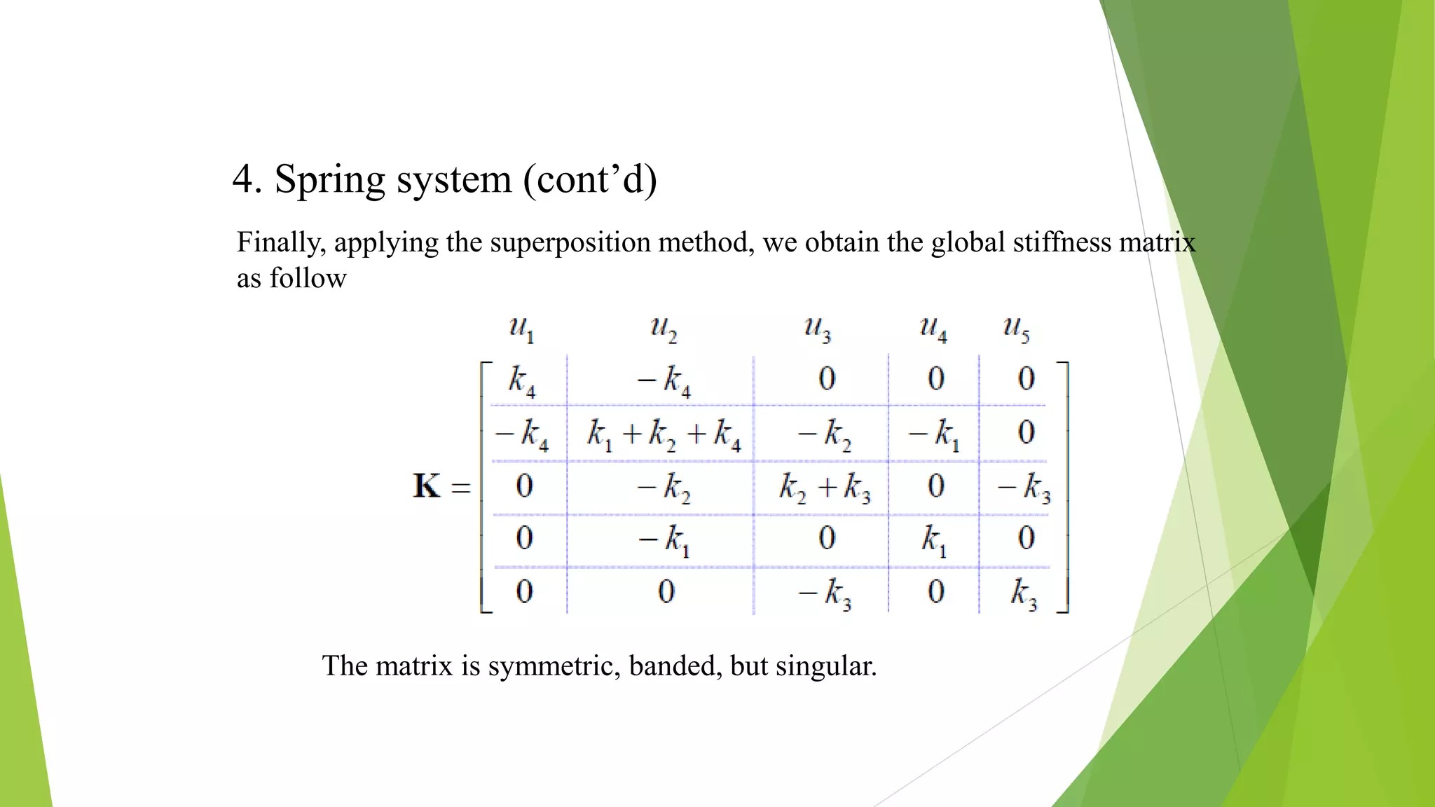
Process of assembling the global stiffness matrix for spring systems, including examples and solutions for specific cases.
Closing remarks and an invitation for questions following the lecture.