Downloaded 55 times


![14
SOLO
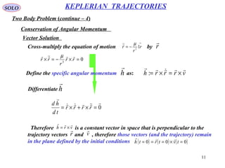
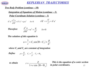
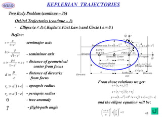
Two Body Problem (continue – 7)
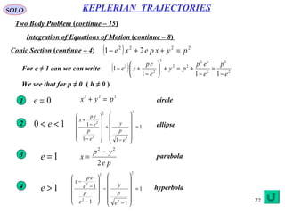
KEPLERIAN TRAJECTORIES
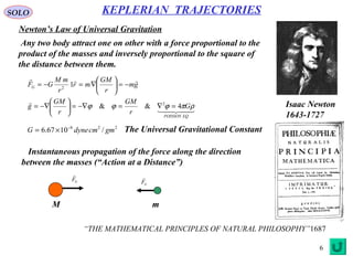
Integration of Equations of Motion
Vector Solution
Cross-multiply the equation of motion with the specific angular momentum
→
−= r
r
r 12
µ
h
hr
r
hr
×−=× 3
µ
( ) ( ) ( )rr
td
d
rhrh
td
d
rhrhr
td
d
××+×=×+×=×
The left side is
( ) ( ) hrr
r
rrhrrrrrrrhr
×=
−××+×=××+××+×=
0
3
0
µ
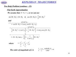
The right side can be written
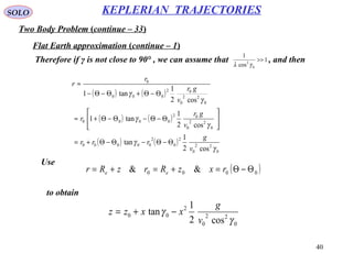
( ) ( ) ( )[ ] ( )
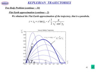
=−=−=⋅−⋅=××−=×−
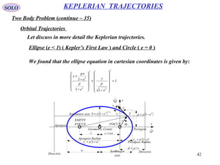
r
r
td
d
r
r
r
v
r
rrrrv
r
vrrrrv
r
vrr
r
hr
r
µ
µµµµµµ
2
2
3333
Equaling both sides gives ( )
=×
r
r
td
d
hr
td
d
µ
Integrating both sides B
r
r
hr
+=× µ
where is the constant of integrationB
](https://image.slidesharecdn.com/kepleriantrajectories-150813153625-lva1-app6891/85/Keplerian-trajectories-14-320.jpg)


![23
SOLO
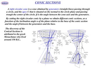
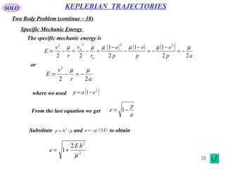
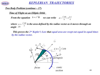
Two Body Problem (continue – 16)
KEPLERIAN TRAJECTORIES
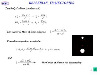
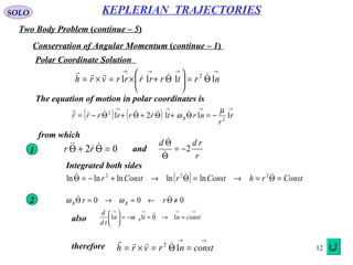
Velocity on the Trajectory
Let find the velocity on the trajectory in and coordinates
→→
tr 1,1
→→
QP 1,1
→→→→
+=Θ+== QyPxtrrrrv 1111
( ) ( )[ ] ( ) ( )[ ]
→→
Θ−ΘΘ+Θ−Θ+Θ−ΘΘ−Θ−Θ= QrrPrr pppp 1cossin1sincos
From the equation of motion
( )pe
p
r
Θ−Θ+
=
cos1 hr =Θ2 µ/: 2
hp =
we obtain ( )
( )[ ]
( )
( )p
p
p
p
r
e
p
p
eh
r
h
e
ep
td
d
d
dr
rv
Θ−Θ=
Θ−Θ
=
Θ−Θ+
Θ−Θ
=
Θ
Θ
==
sin
sin
cos1
sin
22
µ
( )[ ]pt e
pr
p
r
h
rrv Θ−Θ+===Θ= cos12
µµ](https://image.slidesharecdn.com/kepleriantrajectories-150813153625-lva1-app6891/85/Keplerian-trajectories-23-320.jpg)
![24
SOLO
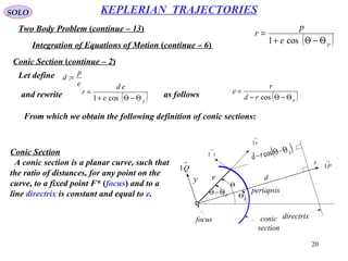
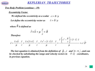
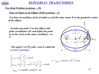
Two Body Problem (continue – 17)
KEPLERIAN TRAJECTORIES
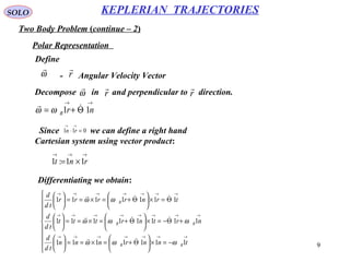
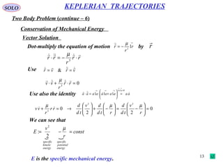
Velocity on the Trajectory (continue – 1)
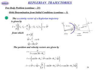
Let substitute those results in the velocity equation to obtain the components
in coordinates.
→→
QP 1,1
( ) ( )[ ]
→→→→
Θ−Θ++Θ−Θ−=+= Qe
p
P
p
QyPxv pp 1cos1sin11
µµ
( ) ( ) ( ) ( )[ ]{ } 2/12222/1222/122
cos1sin pptr ee
p
yxvvv Θ−Θ++Θ−Θ=+=+=
µ
( )[ ] 2/12
cos21 pee
p
v Θ−Θ++=
µ
Θ
pΘ
pΘ−Θ
r d
directrix
focus conic
section
x
y
→
P1
→
Q1
→
r1
→
t1
v
rv tv
periapsis
The velocities at the periapsis
and apoapsis are
( )pΘ=Θ
( )π+Θ=Θ p
( )e
p
va −= 1
µ
( )e
p
vp += 1
µ](https://image.slidesharecdn.com/kepleriantrajectories-150813153625-lva1-app6891/85/Keplerian-trajectories-24-320.jpg)
![30
SOLO
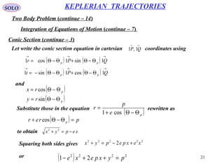
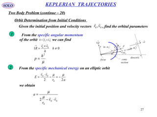
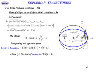
Two Body Problem (continue – 23)
KEPLERIAN TRAJECTORIES
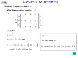
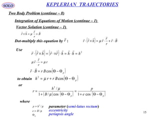
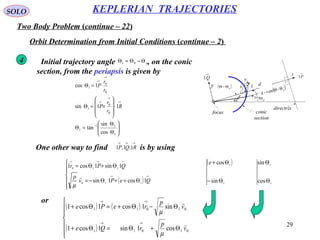
Orbit Determination from Initial Conditions (continue – 3)
Θ pΘr
d
directrix
focus conic
section
x
y
→
P1
→
Q1
→
r1
→
t1
v
rv
tv( )pΘ−Θ γ
Using
1
0
cos1 Θ+
=
e
p
r
we finally obtain
( )
Θ+
Θ
=
Θ−
Θ+
=
→→
→→
01
0
0
1
01
0
0
1
cos
sin
1
sin
cos
1
v
p
r
r
p
Q
v
p
r
r
p
e
P
µ
µ
( )[ ] ( )
( )[ ] ( )
( )[ ] ( ) 01
0
01
01
0
01
011
0
011
sincos11
sincos1cos1
sincoscossinsinsincoscos
1sin1cos
v
p
rr
r
p
r
v
p
rr
re
p
r
v
p
rr
re
p
r
QPrr
Θ−Θ+
Θ−Θ+−=
Θ−Θ+Θ−Θ+−Θ+=
ΘΘ−ΘΘ+ΘΘ+Θ+Θ=
Θ+Θ=
→
→
→
→→
µ
µ
µ
Therefore](https://image.slidesharecdn.com/kepleriantrajectories-150813153625-lva1-app6891/85/Keplerian-trajectories-30-320.jpg)
![31
SOLO
Two Body Problem (continue – 24)
KEPLERIAN TRAJECTORIES
Orbit Determination from Initial Conditions (continue – 4)
Θ pΘr
d
directrix
focus conic
section
x
y
→
P1
→
Q1
→
r1
→
t1
v
rv
tv( )pΘ−Θ γ
where we used
( )
( ) ( ) ( )[ ]
( ) ( )[ ] 011
0
0
11
011
0
0
11
coscos
sinsinsin
coscossinsin
sincoscossin
1cos1sin
ve
p
r
r
p
ee
p
ve
p
r
r
p
ee
p
QeP
p
v
Θ+Θ+Θ+
Θ−Θ−Θ−Θ
=
ΘΘ++ΘΘ+
ΘΘ+−Θ+Θ
−=
Θ++Θ−=
→
→
→→
µ
µ
µ
( ) ( )[ ] ( )
( )[ ]
( )[ ] ( )[ ] ( )[ ]
( )[ ] ( ) ( )[ ] 01
0
01
0
1
0
00
01
0
0
1111
011
0
0
111111
cos11sin
1
cos1
cos11
cos1sincos1sin
cos1cos1
sinsincoscossinsin
v
p
r
r
pr
e
pr
vr
v
p
r
r
p
eee
p
ve
p
r
r
p
ee
p
Θ+Θ−−+
Θ−Θ−Θ−Θ−
⋅
=
Θ+Θ−−+
Θ+Θ−Θ−Θ−Θ−Θ
=
Θ++Θ+Θ+−+
Θ−Θ−Θ−ΘΘ+Θ−ΘΘ−Θ
=
→
→
→
→
µ
µ
µ
( )
10
1111000
sin
1cos1sin1sin1cos
Θ=
Θ++Θ−⋅
Θ+Θ=⋅
→→→→
e
p
r
QeP
p
QPrvr
µ
µ](https://image.slidesharecdn.com/kepleriantrajectories-150813153625-lva1-app6891/85/Keplerian-trajectories-31-320.jpg)
![32
SOLO
Two Body Problem (continue – 25)
KEPLERIAN TRAJECTORIES
Orbit Determination from Initial Conditions (continue – 5)
Θ pΘr
d
directrix
focus conic
section
x
y
→
P1
→
Q1
→
r1
→
t1
v
rv
tv( )pΘ−Θ γ
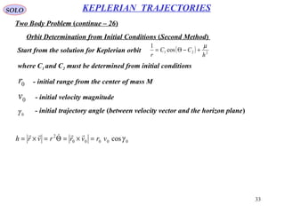
Summarize
( )[ ] ( ) 01
0
01 sincos11 v
p
rr
r
p
r
r
Θ−Θ+
Θ−Θ+−=
→
µ
( )[ ] ( ) ( )[ ] 01
0
01
0
1
0
00
cos11sin
1
cos1 v
p
r
r
pr
e
pr
vr
v
Θ+Θ−−+
Θ−Θ−Θ−Θ−
⋅
=
→
→
µ](https://image.slidesharecdn.com/kepleriantrajectories-150813153625-lva1-app6891/85/Keplerian-trajectories-32-320.jpg)
![35
SOLO
Two Body Problem (continue – 28)
KEPLERIAN TRAJECTORIES
Orbit Determination from Initial Conditions (Second Method - 2)
We have
( )
0
2
00
201
cos
11
cos
γλ rr
CC −=−Θ
( ) 0
0
201 tan
1
sin γ
r
CC =−Θ
( ) ( )[ ]
( ) ( ) ( ) ( )
( ) ( )
0
2
0
00
0
0
0
2
00
0
2
0
02010201
0
2
0
2001
cos
1
sintan
1
cos
cos
11
cos
1
sinsincoscos
cos
1
cos
1
γλ
γ
γλ
γλ
γλ
rrrr
r
CCCC
r
CC
r
+Θ−Θ−Θ−Θ
−=
+Θ−Θ−Θ−Θ−Θ−Θ=
+−Θ+Θ−Θ=
( ) ( ) ( )
( ) ( )
0
00
0
2
0
0
0000
0
2
00
cos
cos
cos
cos1
cos
sinsincoscos
cos
cos1
γ
γ
γλ
γ
γγ
γλ
+Θ−Θ
+
Θ−Θ−
=
Θ−Θ−Θ−Θ
+
Θ−Θ−
=
r
r
which, when developed further, gives](https://image.slidesharecdn.com/kepleriantrajectories-150813153625-lva1-app6891/85/Keplerian-trajectories-35-320.jpg)

![37
SOLO
Two Body Problem (continue – 30)
KEPLERIAN TRAJECTORIES
Orbit Determination from Initial Conditions (Second Method - 3)
( ) ( )0000
0
2
0
coscoscos1
cos
γγλ
γλ
+Θ−Θ+Θ−Θ−
=
r
r
( ) ( )
( ) ( ) ( )
( ) ( ) ( ) ( )[ ]
( )2
0
2
0
2
0
22
00
2
0002
0
2
0
2
0
22
00
2
000
0000
1coscossin
cos1cossincossin
1coscossin1
cos1cossincossin1
coscoscos1
−+
Θ−Θ−+Θ−Θ−
−++=
Θ−Θ−+Θ−Θ−=
+Θ−Θ+Θ−Θ−
γλγγλ
γλγγλ
γλγγλ
γλγγλ
γγλ
The denominator can be expressed as
0
2
0 cos: γλrp =
( ) ( ) 1cos21cos2cos1coscossin: 0
2
0
2
0
222
0
2
0
2
0
22
+−=+−=−+= γλλγλγλγλγγλe
We define
−
=Θ−Θ −
1cos
cossin
tan:
0
2
001
0
γλ
γγλ
p
( ) ( )
( ) ( )[ ] ( )pp
ee Θ−Θ+=Θ−Θ+Θ−Θ+=
+Θ−Θ+Θ−Θ−
cos1cos1
coscoscos1
00
0000
γγλto obtain](https://image.slidesharecdn.com/kepleriantrajectories-150813153625-lva1-app6891/85/Keplerian-trajectories-37-320.jpg)
![38
SOLO
Two Body Problem (continue – 31)
KEPLERIAN TRAJECTORIES
Orbit Determination from Initial Conditions (Second Method - 4)
( ) ( )0000
0
2
0
coscoscos1
cos
γγλ
γλ
+Θ−Θ+Θ−Θ−
=
r
r
The denominator can be expressed as
( ) ( ) ( ) ( )[ ] ( )pp
ee Θ−Θ+=Θ−Θ+Θ−Θ+=+Θ−Θ+Θ−Θ− cos1cos1coscoscos1 000000
γγλ
We obtain again the fact that the trajectory is a conic section given by
( )pe
p
r
Θ−Θ+
=
cos1
We can also write
( )[ ] λγλλ
γλ
−
=
+−−
=
−
=
21cos21
cos
1
: 0
0
2
0
2
0
2
rr
e
p
a
and
0
2
0 cos: γλrp = ( ) 1cos2: 0
2
+−= γλλe](https://image.slidesharecdn.com/kepleriantrajectories-150813153625-lva1-app6891/85/Keplerian-trajectories-38-320.jpg)

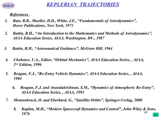
![48
SOLO
Two Body Problem (continue – 41)
KEPLERIAN TRAJECTORIES
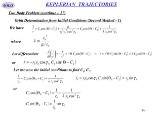
Time of Flight on an Elliptic Orbit (continue – 4)
From
x
y
eac =
a a
( ) 2/12
1 eab −=
rΘ
FOCUS
EMPTY
FOCUS
c
→
P1
→
Q1
a
F
Q
O VS
E
P
Eeary
aeEarx
ellipse
ellipse
sin1sin
coscos
2
−=Θ=
−=Θ=
we have
( ) ( )[ ] [ ]
( )Eea
EeEeaEeaaeEar
cos1
coscos21sin1cos
2/1222/12222
−=
+−=−+−=
Therefore
Θ+
Θ−
=
−
−
=Θ
Θ+
Θ+
=
−
−
=Θ
cos1
sin1
sin
cos1
sin1
sin
cos1
cos
cos
cos1
cos
cos
22
e
e
E
Ee
Ee
e
e
E
Ee
eE
( )( )
Ee
Ee
Ee
eEEe
sin1
cos11
sin1
coscos1
sin
cos1
2
tan
22
−
−+
=
−
+−−
=
Θ
Θ−
=
Θ
From
2
tan
1
1
2
tan
E
e
e
−
+
=
Θ
or
and are always in the same quadrant.2
Θ
2
E](https://image.slidesharecdn.com/kepleriantrajectories-150813153625-lva1-app6891/85/Keplerian-trajectories-48-320.jpg)


The document discusses Kepler's laws of planetary motion and Newton's laws of motion and universal gravitation, providing insights on the two-body problem and its mathematical implications. It elaborates on various concepts including conservation of angular momentum, mechanical energy, and the integration of equations of motion relevant to orbital trajectories. The document serves as a comprehensive guide to understanding the dynamics of celestial bodies and their orbits.