Downloaded 391 times
![SOLO Lead Computing Gunsight
A gyro gunsight (G.G.S.) is a modification of the non-magnifying
reflector sight in which target lead (the amount of aim-off in front of a
moving target) and bullet drop are allowed for automatically, the sight
incorporating a gyroscopic mechanism that computes the necessary
deflections required to ensure a hit on the target. The sight was developed
just before the Second World War for aircraft use during aerial combat.
Gyro Gunsight (G.G.S.)
The Ferranti Gyro Sight Mk IIc
Gyro gunsights were (for the most part) modifications of the reflector
gunsight to aid pilots in hitting targets (other aircraft) that were turning
rapidly in front of them. The reflector sight (first used on German
fighters in 1918[1]
and widely adopted on all kinds of fighter and bomber
aircraft in the 1930s) was an optical device consisting of a 45 degree
angle glass beam splitter that sat in front of the pilot and projected an illuminated image of an
aiming reticule that appeared to sit out in front of the pilot's field of view at infinity and was
perfectly aligned with the plane's guns ("boresighted" with the guns). The optical nature of the
reflector sight meant it was possible to feed other information into field of view, such as
modifications of the aiming point due to deflection determined by input from a gyroscope.[2]
It is important to note that the information presented to the pilot was of his own aircraft, that is
the deflection/lead calculated was based on his own bank-level, rate of turn, airspeed etc. The
assumption was that the flight-path was following the flight-path of the target aircraft, as in a
dogfight, therefore the input data was close-enough
History
Optical system of Gyro Sight](https://image.slidesharecdn.com/6-computinggunsighthudandhms-150812123017-lva1-app6892/75/6-computing-gunsight-hud-and-hms-4-2048.jpg)
![SOLO Lead Computing Gunsight
Gyro Gunsight (G.G.S.)
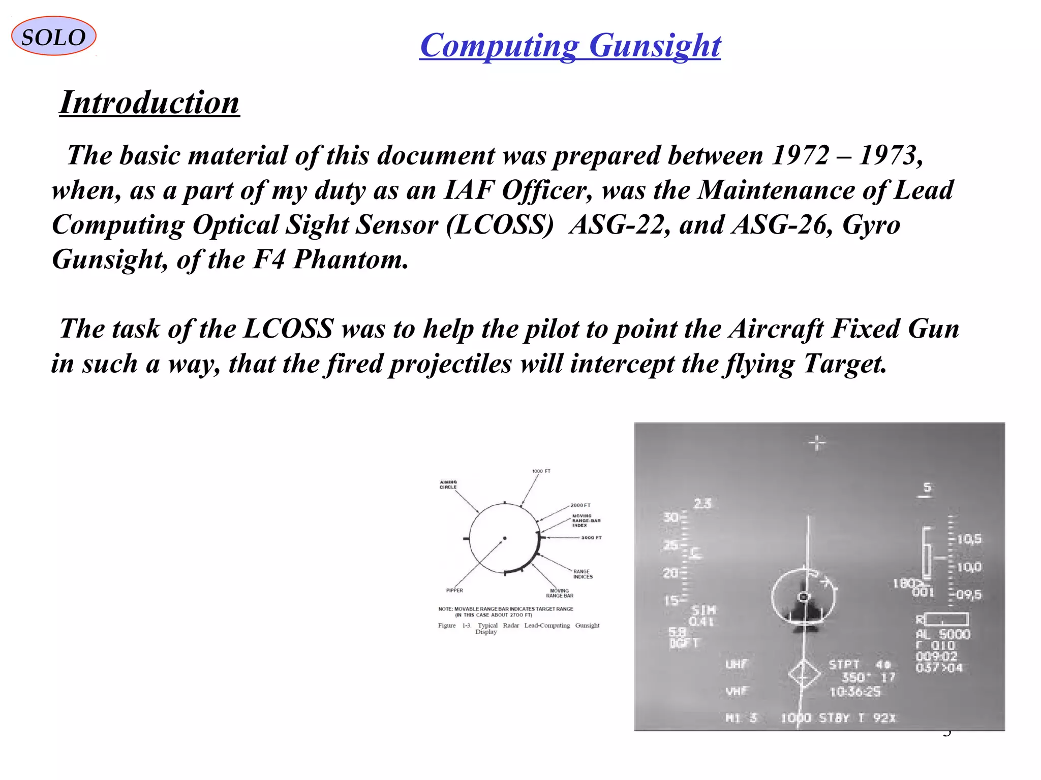
History (continue – 1)
After tests with two experimental gyro gunsights which had begun in 1939, the first production
gyro gunsight was the British Mark I Gyro Sight , developed at Farnborough in 1941. To save
time in development the sight was based on the already existing type G prismatic sight, basically a
telescopic gun sight folded into a shorter length by a series of prisms.[3]
Prototypes were tested in
a Supermarine Spitfire and the turret of a Boulton Paul Defiant in the early part of that year.
With the successful conclusion of these tests the sight was put into production by Ferranti, the
first limited-production versions being available by the spring of 1941, with the sights being first
used operationally against Luftwaffe raids on Britain in July the same year. The Mark I sight
had a number of drawbacks however, including a limited field of view, erratic behavior of the
reticle, and requiring the pilot/gunner to put their eye up against an eyepiece during violent
maneuvers.
Production of the Mark I was postponed and work started on an improved sight. Changes
involved incorporating the gyro adjusted reticle into a more standard reflector sight system. This
new sight became the Mark II Gyro Sight, which was first tested in late 1943 with production
examples becoming available later in the same year. In the Mark II the pilot had to set the
wingspan of the target, and use a throttle mounted control to keep the target centered
British Developments
The Mark II was also subsequently produced in the US by Sperry as the K-14 (USAAF) and Mk18
(Navy)
The radar-aimed AGLT Village Inn tail turret incorporated a Mark II Gyro Sight and this turret
was fitted to some Lancaster bombers towards the end of World War II.](https://image.slidesharecdn.com/6-computinggunsighthudandhms-150812123017-lva1-app6892/75/6-computing-gunsight-hud-and-hms-5-2048.jpg)
![SOLO Lead Computing Gunsight
Gyro Gunsight (G.G.S.)
History (continue – 3)
German Developments
Although since 1935 the relevant German companies offered the Reich Air Ministry (RLM) a new type of gyro-
stabilized sight, the well-proven REVI (Reflexvisier, or reflector sight) remained in service for combat aircraft. The
gyro-stabilized sights received an additional designation of EZ (Einheitszielvorrichtung, or Target Predictor Units),
such as EZ/REVI-6a. The development of the EZ 40 gyro sight began in 1935 at the Carl Zeiss and Askania
companies, but was of low priority. Not until the beginning of 1942, when a US P-47 Thunderbolt fighter equipped
with a gyro-stabilised sight was captured, did the RLM speed up research. In the summer of 1941, the EZ 40, for
which both the Carl Zeiss and Askania companies were submitting their developments, was rejected. Tested in a Bf
109 F, Askania's EZ 40 produced 50 to 100% higher hit probability compared to the then standard sight, the REVI
C12c.[5]
In the summer of 1943 an example of the EZ 41 developed by the Zeiss company was tested, but was refused
because of too many faults. In the summer 1942, the Askania company began work on the EZ 42, which gunsight
could be adjusted for the target's wingspan (in order to estimate distance to the target). Three examples of the first
series of 33 pieces were delivered in July 1944. These were followed by further 770 units, the last being delivered by
the beginning of March 1945. Each unit took 130 labour hours to produce. The EZ 42 was made up by two major
parts, and lead computation was provided by two gyroscopes. The system, weighing 13.6 kg (30 lb) complete, of which
the reflector sight was 3.2 kg, was ordered into mass production at the Steinheil company in Munich. Approximately
200 of the sights were installed into Fw 190 and Me 262 fighters for field testing. The pilots reported that attacks from
20 degrees deflection were possible, and that although the maximum range of the EZ 42 was stated as approximately
1,000 meters, several enemy aircraft were shot down from a combat distance of 1,500 meters.[6]
The EZ 42 was compared with the Allied G.G.S. captured from in a P-47 Thunderbolt in September 1944 in Germany.
Both sights were tested in the same Fw 190, and by the same pilot. The conclusion was critical of the moving graticule
of the G.G.S., which could be obscured by the target. Compared to the EZ 42, the Allied sight's prediction angle was
found on average to be 20% less accurate, and vary by 1% per degree. Tracking accuracy with the G.G.S. measured as
the mean error of the best 50% of pictures was 20% worse than with the EZ 42
The German [HD], Movie](https://image.slidesharecdn.com/6-computinggunsighthudandhms-150812123017-lva1-app6892/75/6-computing-gunsight-hud-and-hms-7-2048.jpg)
![SOLO Lead Computing Gunsight
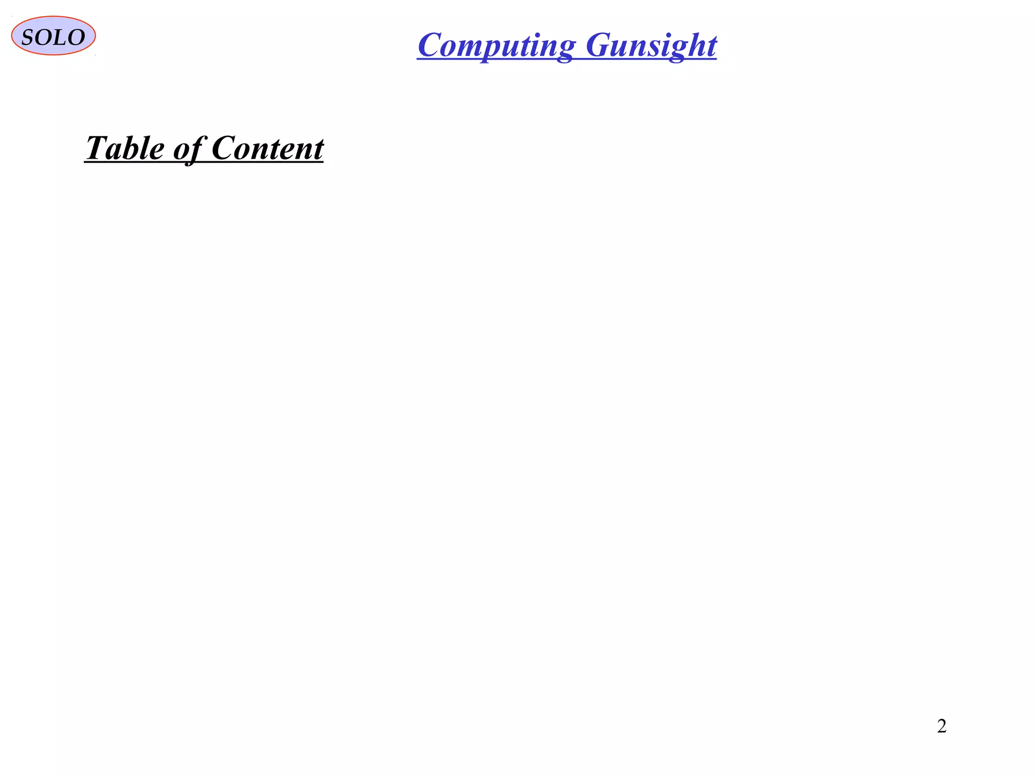
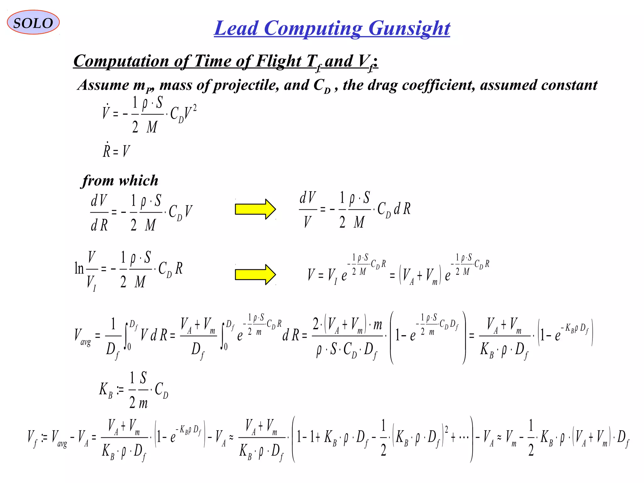
Computation of Time of Flight Tf and Vf (continue – 1)
( ) fmABmAavgf DVVKVVVV ⋅+⋅⋅⋅−≈−= ρ
2
1
:
( ) ∫∫ +=+=
ff T
TS
T
Zf tdVDtdgVD
00
11
( ) ffAfavg
T
f TVVTVtdVD
f
⋅+=⋅=≈ ∫0
( ) fA
T
SSA
T
TSf TDVDtdDDVDtdVDD
ff
⋅++≈
+++≈+= ∫∫
00
111
( ) ( ) ( ) 0=−⋅−⇒⋅++≈⋅+≈ DTDVTDVDTVVD fffAffAf
( ) ( )[ ] 0
2
1
=−⋅
−⋅++⋅+⋅⋅⋅− DTDTDVDVVKV f
D
fAmABm
f
ρ](https://image.slidesharecdn.com/6-computinggunsighthudandhms-150812123017-lva1-app6892/75/6-computing-gunsight-hud-and-hms-15-2048.jpg)
![SOLO Lead Computing Gunsight
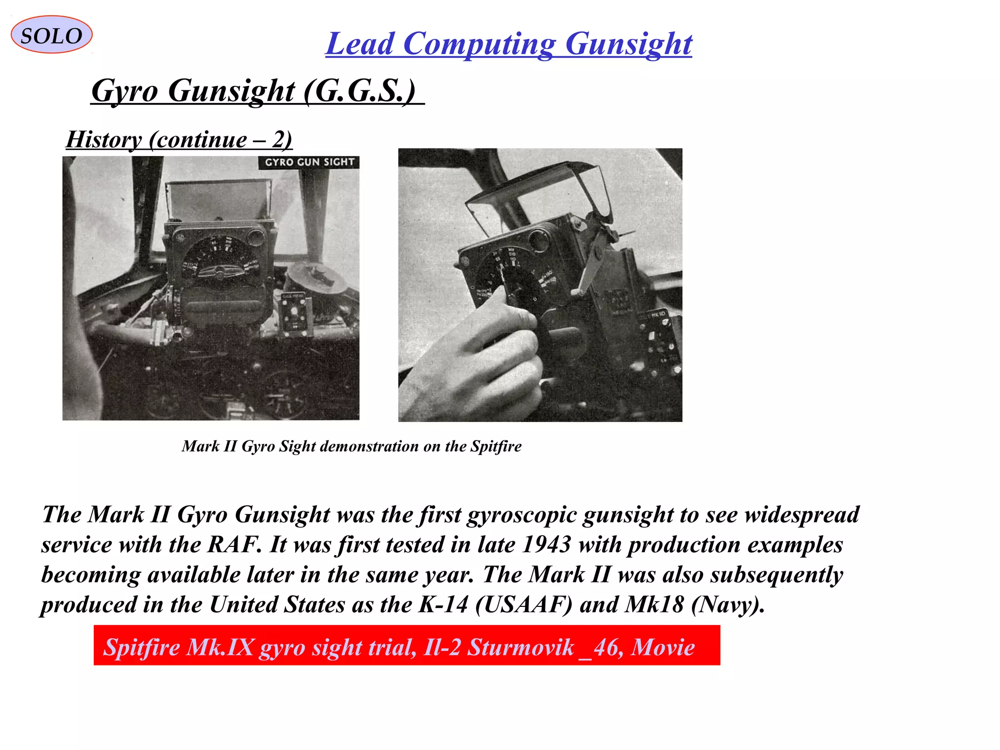
Computation of Time of Flight Tf and Vf (continue – 2)
( ) ( )[ ] 0
2
1
=−⋅
−⋅++⋅+⋅⋅⋅− DTDTDVDVVKV f
V
D
fAmABm
f
f
ρ
( ) ( ) ( ) 0
2
1
2
1 2
=+⋅
+⋅⋅⋅−−⋅+⋅+⋅⋅⋅ DTVVKVTDVVVK f
B
mABmf
A
AmAB
ρρ
A
DABB
Tf
⋅
⋅⋅−−
=
2
42
ff TDDV /+= ](https://image.slidesharecdn.com/6-computinggunsighthudandhms-150812123017-lva1-app6892/75/6-computing-gunsight-hud-and-hms-16-2048.jpg)
![SOLO Lead Computing Gunsight
Gyro Gunsight (G.G.S.)
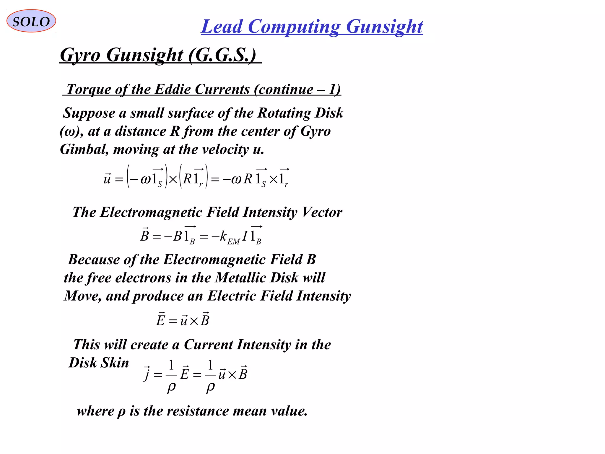
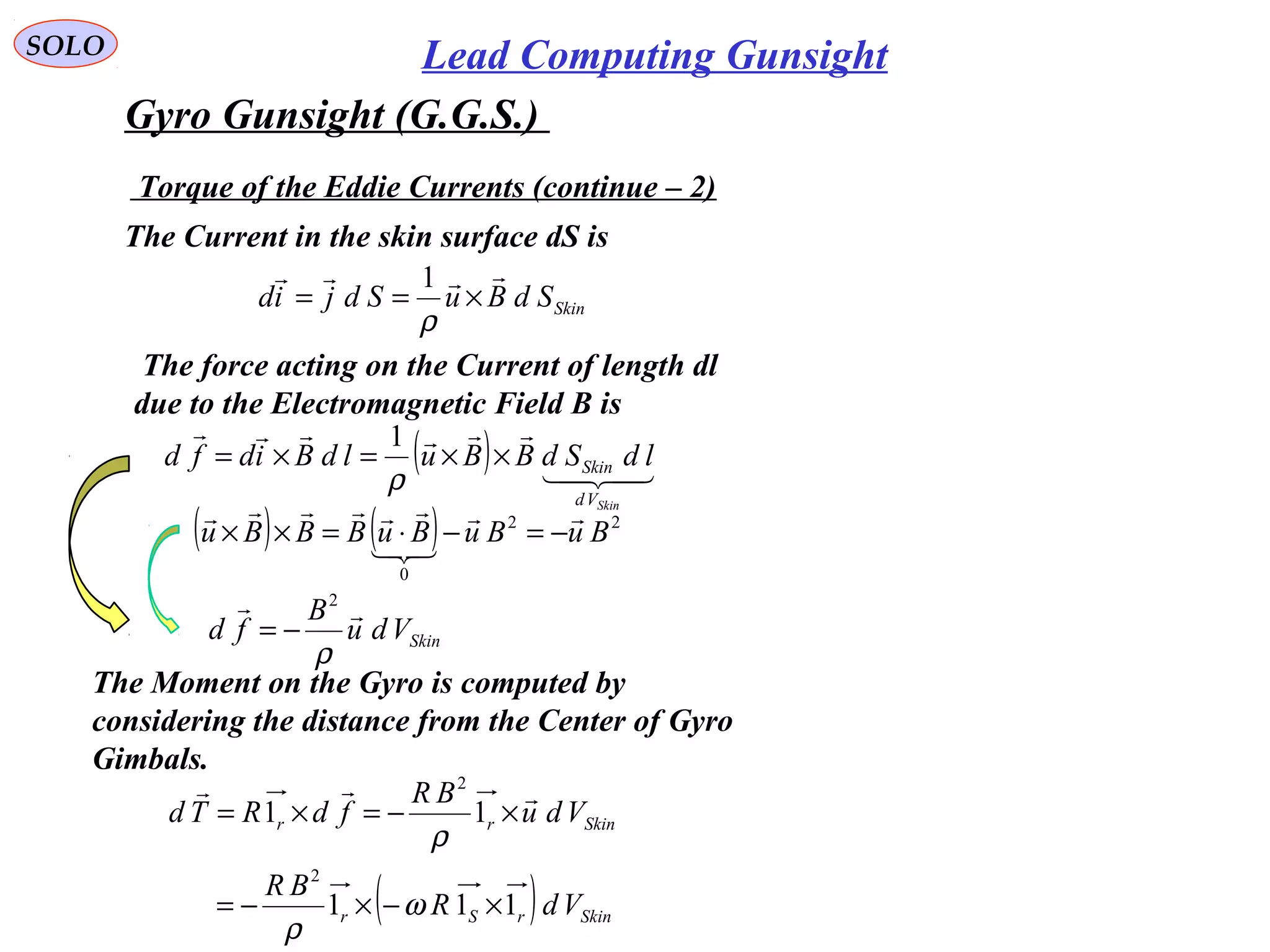
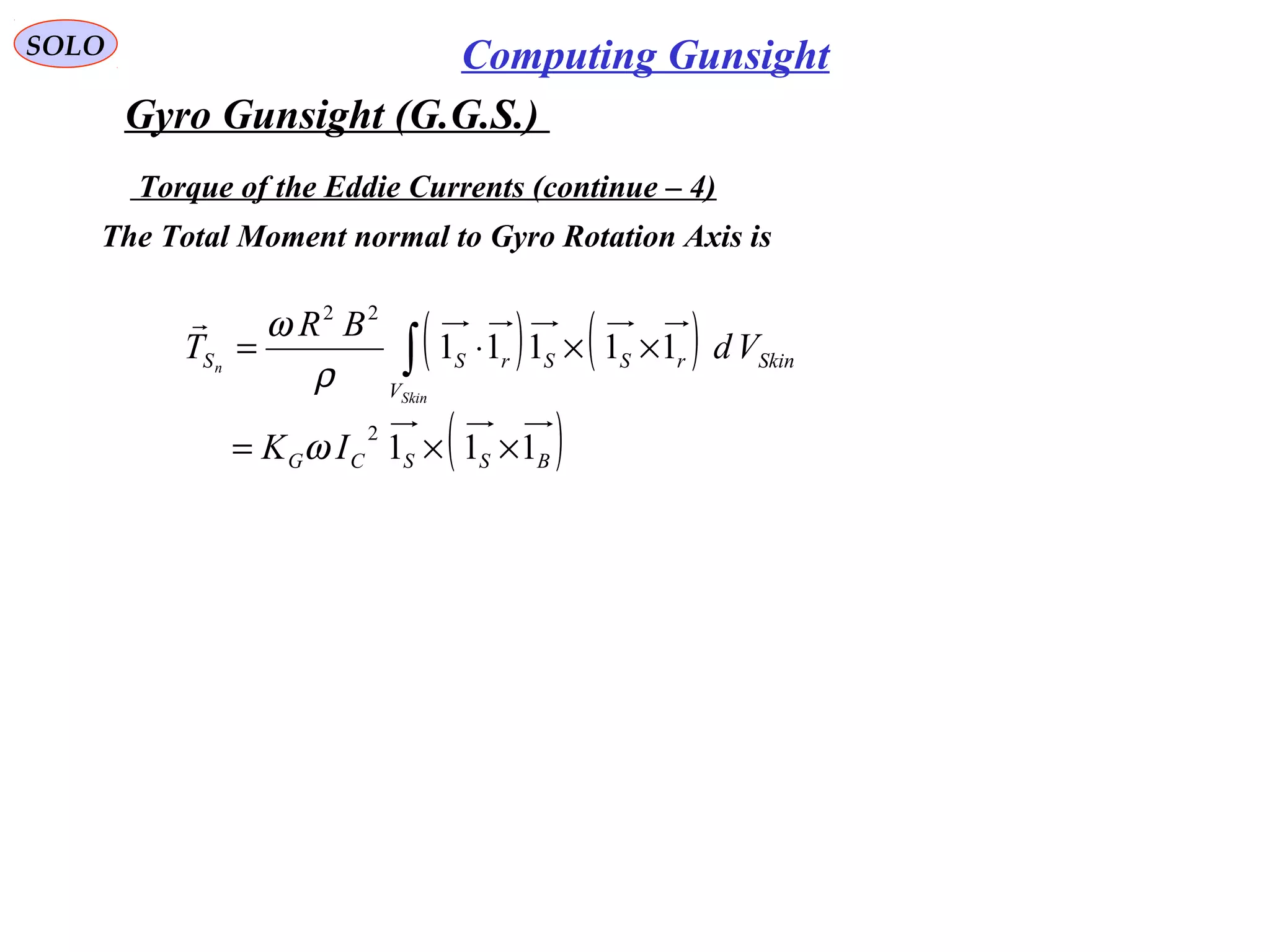
Torque of the Eddie Currents (continue – 3)
( ) SkinrSr Vd
BR
Td 111
22
××=
ρ
ω
( ) ( )
( ) ( )
( ) ( ) ( ) ( )[ ]
( ) ( )
( ) ( ) ( ) ( )rSSrSrSSrSr
rSSrS
rrSSrSrSSrSrS
rSrSrS
rSrSrSr
111111111111
11111
11111111111111
1111111
1111111
2
2
2
××⋅+
⋅−=××
××⋅=
−⋅⋅=
⋅−−⋅−
⋅−=××⋅
⋅−=××
Decompose this in the component in direction
(that will be compensate by the Gyro Motor) and
that normal to it (that will cause the precession).
S1
( ) ( ) ( )
nSS Td
SkinrSSrS
Td
SkinrSS Vd
BR
Vd
BR
Td 111111111
22222
××⋅+
⋅−=
ρ
ω
ρ
ω](https://image.slidesharecdn.com/6-computinggunsighthudandhms-150812123017-lva1-app6892/75/6-computing-gunsight-hud-and-hms-28-2048.jpg)
![SOLO Computing Gunsight
Gyro Gunsight (G.G.S.)
⋅
⋅
−⋅
=×
⋅
⋅−⋅
+
−
⋅+−=Λ
ΛΛ
Λ
SnapShootT
Lead
D
TV
V
D
Ka
V
T
KV
V
VV
VV
K
L
K
f
fA
fNS
f
f
f
A
Am
fm
2
1
1
2
111
32
1
α
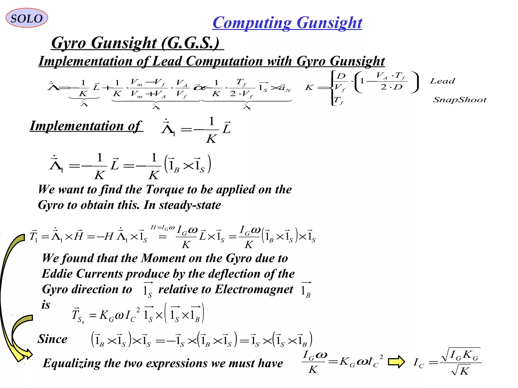
Implementation of
We want to find the Torque to be applied on the
Gyro to obtain this.
( )[ ] SABSGSG
K
K
IIT 1111122
×−×−=×Λ−= α
ωω
( )ABS
K
f
A
Am
fm
K
K
V
V
VV
VV
K
111
1
:2
−×=⋅
+
−
⋅=Λ α
α
α
( )[ ]
( )
αωω α
α
α
K
K
I
K
K
IT GSABSG
ABS
=×−×=
≈−
11,1sin
2 1111
( )ABS 111:
−×=α
f
A
Am
fm
V
V
VV
VV
K ⋅
+
−
=:α
Implementation of Lead Computation with Gyro Gunsight (continue – 1)](https://image.slidesharecdn.com/6-computinggunsighthudandhms-150812123017-lva1-app6892/75/6-computing-gunsight-hud-and-hms-31-2048.jpg)
![SOLO Computing Gunsight
Gyro Gunsight (G.G.S.)
⋅
⋅
−⋅
=×
⋅
⋅−⋅
+
−
⋅+−=Λ
ΛΛ
Λ
SnapShootT
Lead
D
TV
V
D
Ka
V
T
KV
V
VV
VV
K
L
K
f
fA
fNS
f
f
f
A
Am
fm
2
1
1
2
111
32
1
α
( ) SNS
f
f
GSG a
V
T
K
IIT 11
2
1
133
××
⋅
⋅=×Λ−= ωω
Implementation of Lead Computation with Gyro Gunsight (continue – 3)
is perpendicular to and in the plane defined
by and
S1
( )AB 11
−
S1
is perpendicular to and in the plane defined
by and
S1
Na
S1
Since L and α are small angles, we may say
that and are collinear and in the
Gyro zG direction, therefore
2T
3T
GGG Z
f
NfG
ZZ
V
aT
K
K
I
TTT 1
2
132
⋅
⋅
+−=≈+ α
ω
α
( )[ ] SABSGSG
K
K
IIT 1111122
×−×−=×Λ−= α
ωω](https://image.slidesharecdn.com/6-computinggunsighthudandhms-150812123017-lva1-app6892/75/6-computing-gunsight-hud-and-hms-33-2048.jpg)
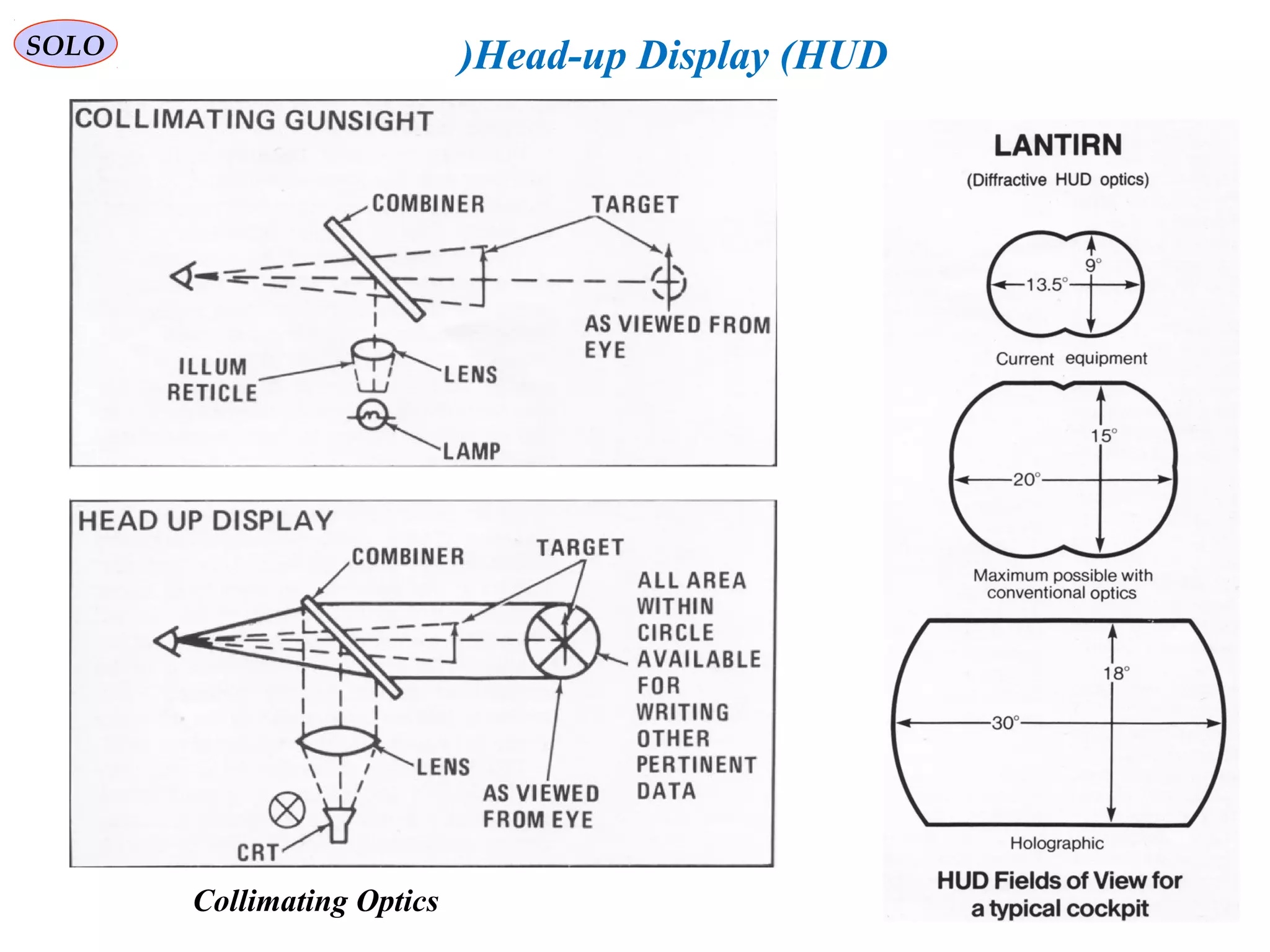
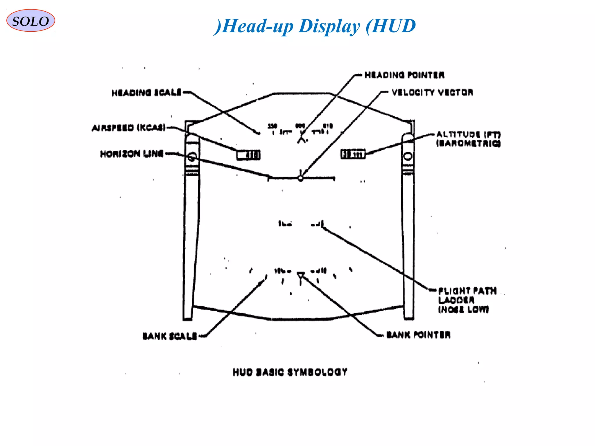
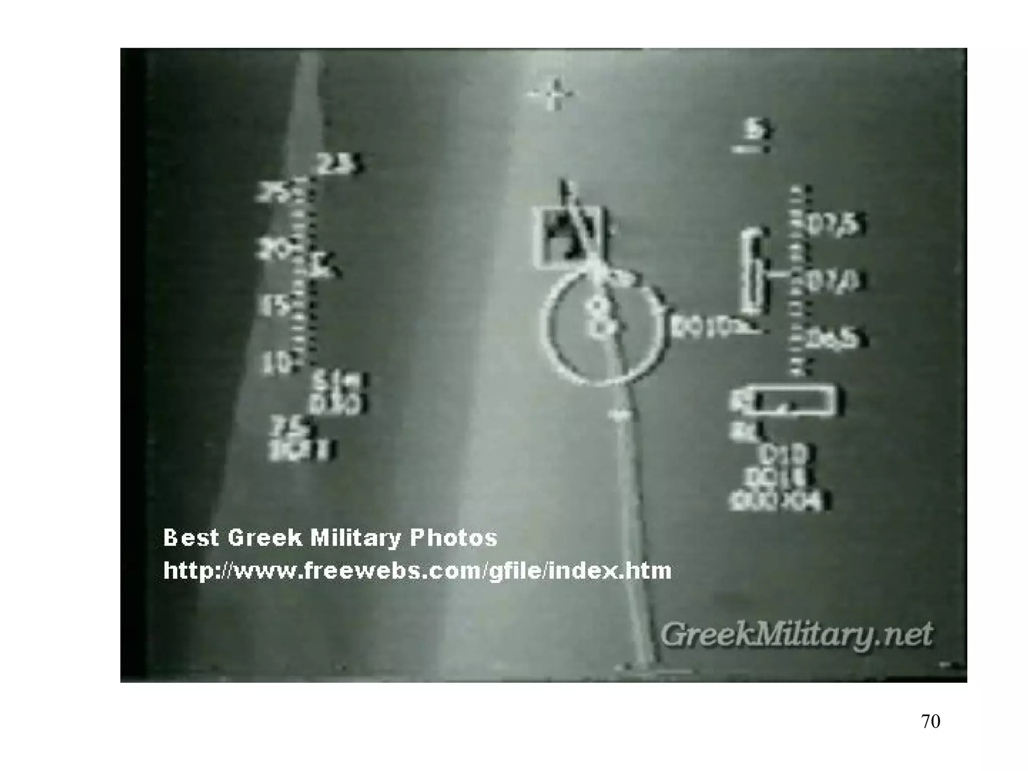
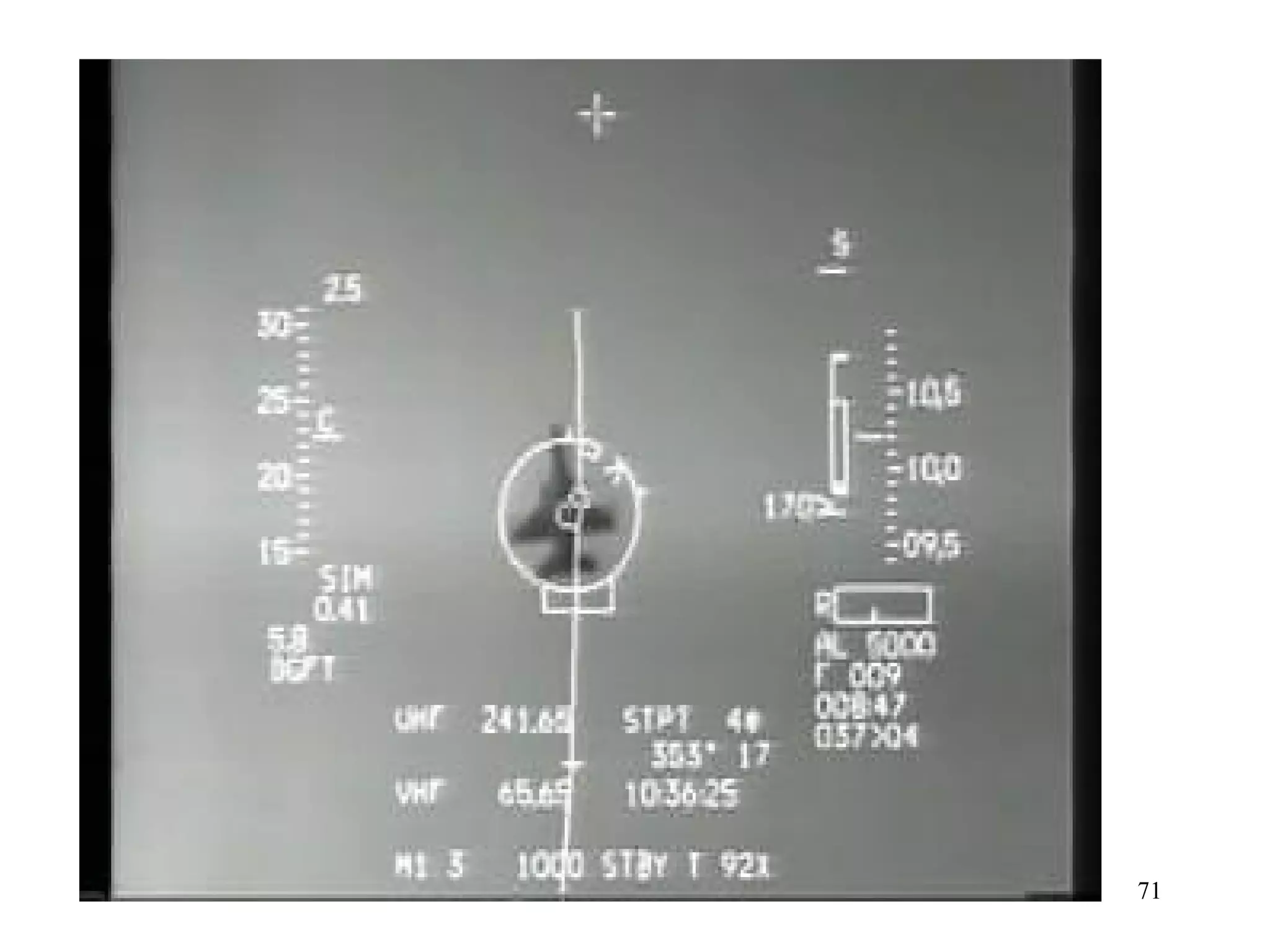
![SOLO Head-up Display (HUD(
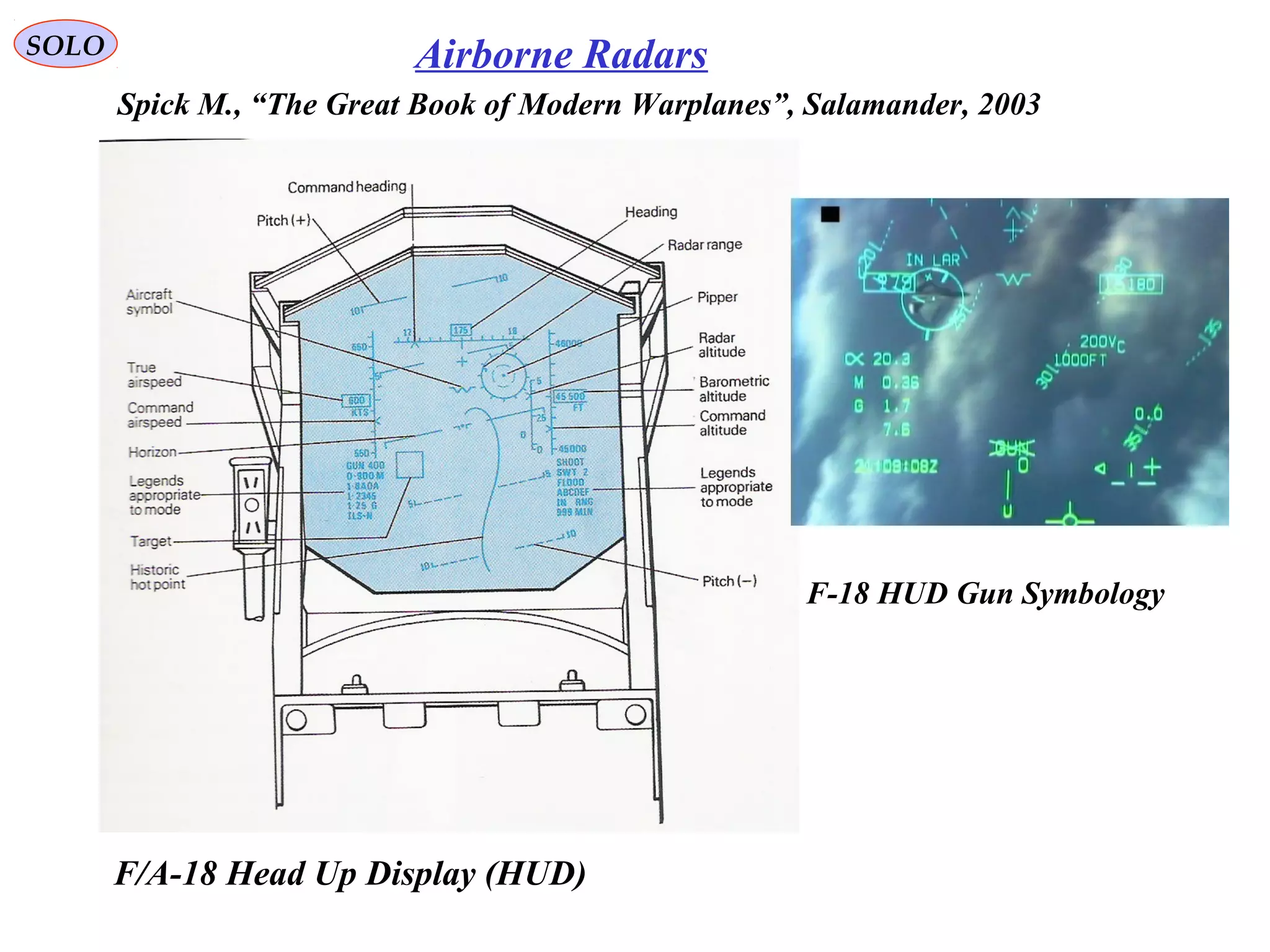
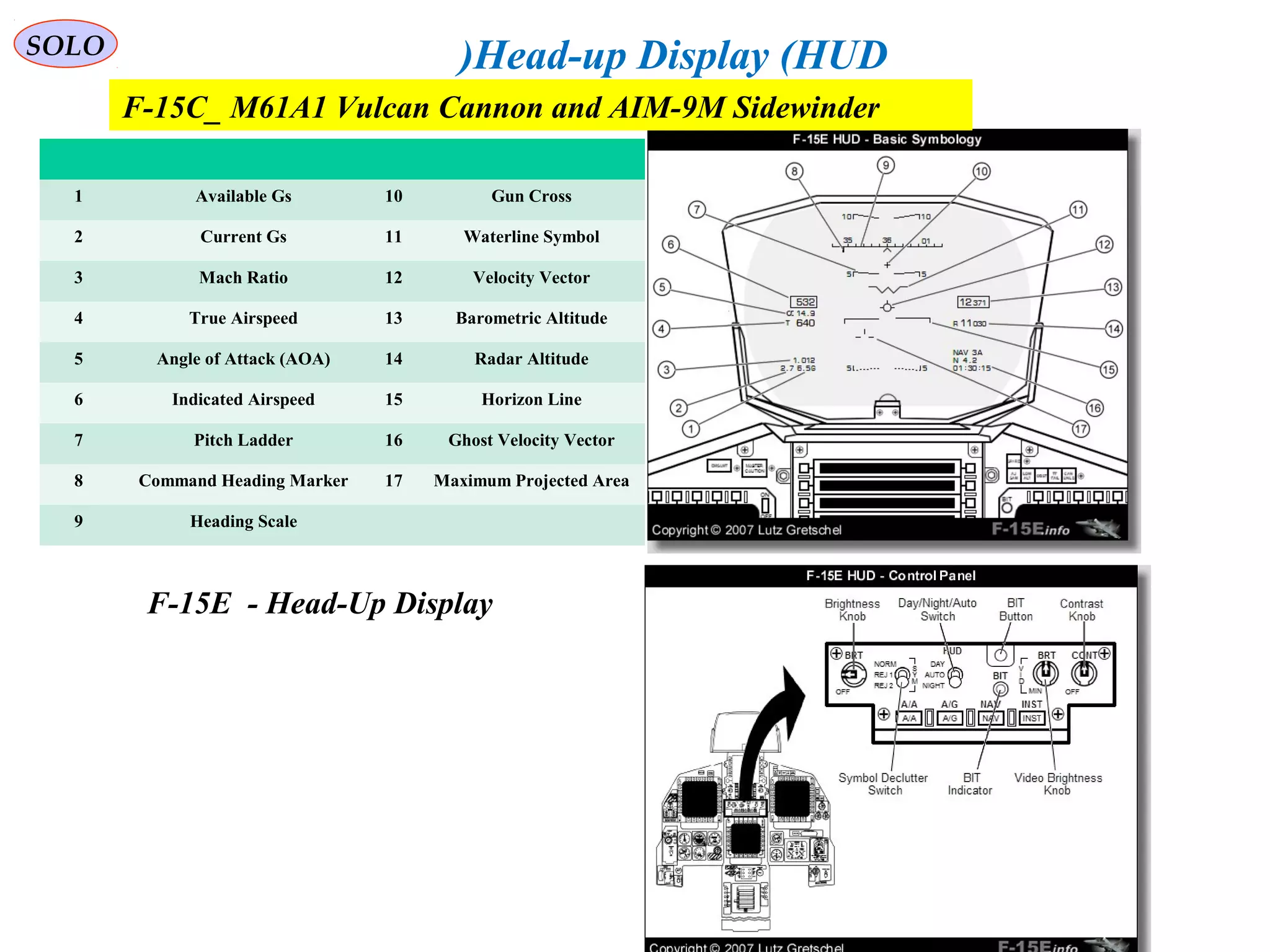
Typical aircraft HUDs display data: Airspeed, Altitude, a Horizon Line, Heading,
Turn/Bank and Slip/Skid indicators. These instruments are the minimum required by
14 CFR Part 91.
Other symbols and data are also available in some HUDs:
• Boresight or Waterline Symbol —is fixed on the display and shows where the nose
of the aircraft is actually pointing.
• Flight Path Vector (FPV( or Velocity Vector Symbol —shows where the aircraft is
actually going, the sum of all forces acting on the aircraft.]
For example, if the aircraft
is pitched up but is losing energy, then the FPV symbol will be below the horizon even
though the boresight symbol is above the horizon. During approach and landing, a
pilot can fly the approach by keeping the FPV symbol at the desired descent angle and
touchdown point on the runway.
• Acceleration Indicator or Energy Cue —typically to the left of the FPV symbol, it is
above it if the aircraft is accelerating, and below the FPV symbol if decelerating.
• Angle Of Attack indicator —shows the wing's angle relative to the airflow, often
displayed as "α".
• Navigation Data and Symbols —for approaches and landings, the flight guidance
systems can provide visual cues based on navigation aids such as an Instrument
Landing System (ILS( or Augmented Global Positioning System such as the Wide
Area Augmentation System. Typically this is a circle which fits inside the flight path
vector symbol. Pilots can fly along the correct flight path by "flying to" the guidance
cue.](https://image.slidesharecdn.com/6-computinggunsighthudandhms-150812123017-lva1-app6892/75/6-computing-gunsight-hud-and-hms-43-2048.jpg)

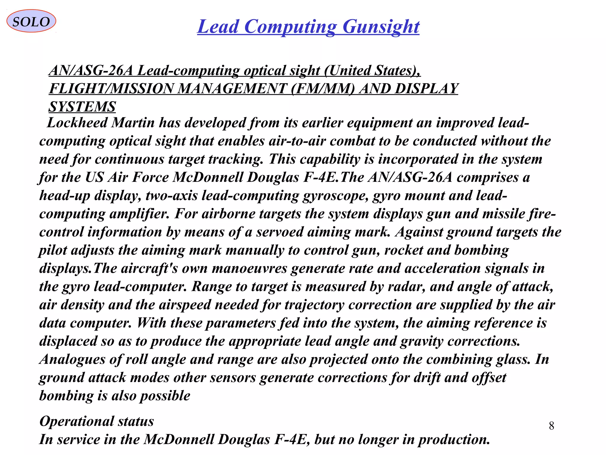
The document summarizes the history and development of gyro gunsights used in aircraft from World War 2 through the Cold War. Gyro gunsights automatically calculated the lead angle and bullet drop needed for a pilot to hit a moving target. The first operational gyro gunsight was the British Mark I in 1941. Improved models like the Mark II saw widespread use through the end of WWII. Germany developed the EZ 42 gyro sight but it did not see full deployment. The US developed the AN/ASG-26 for the F-4 Phantom, which provided targeting information via a head-up display.


