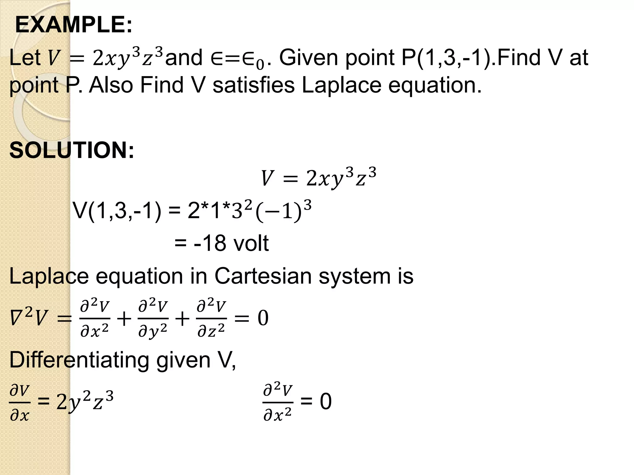
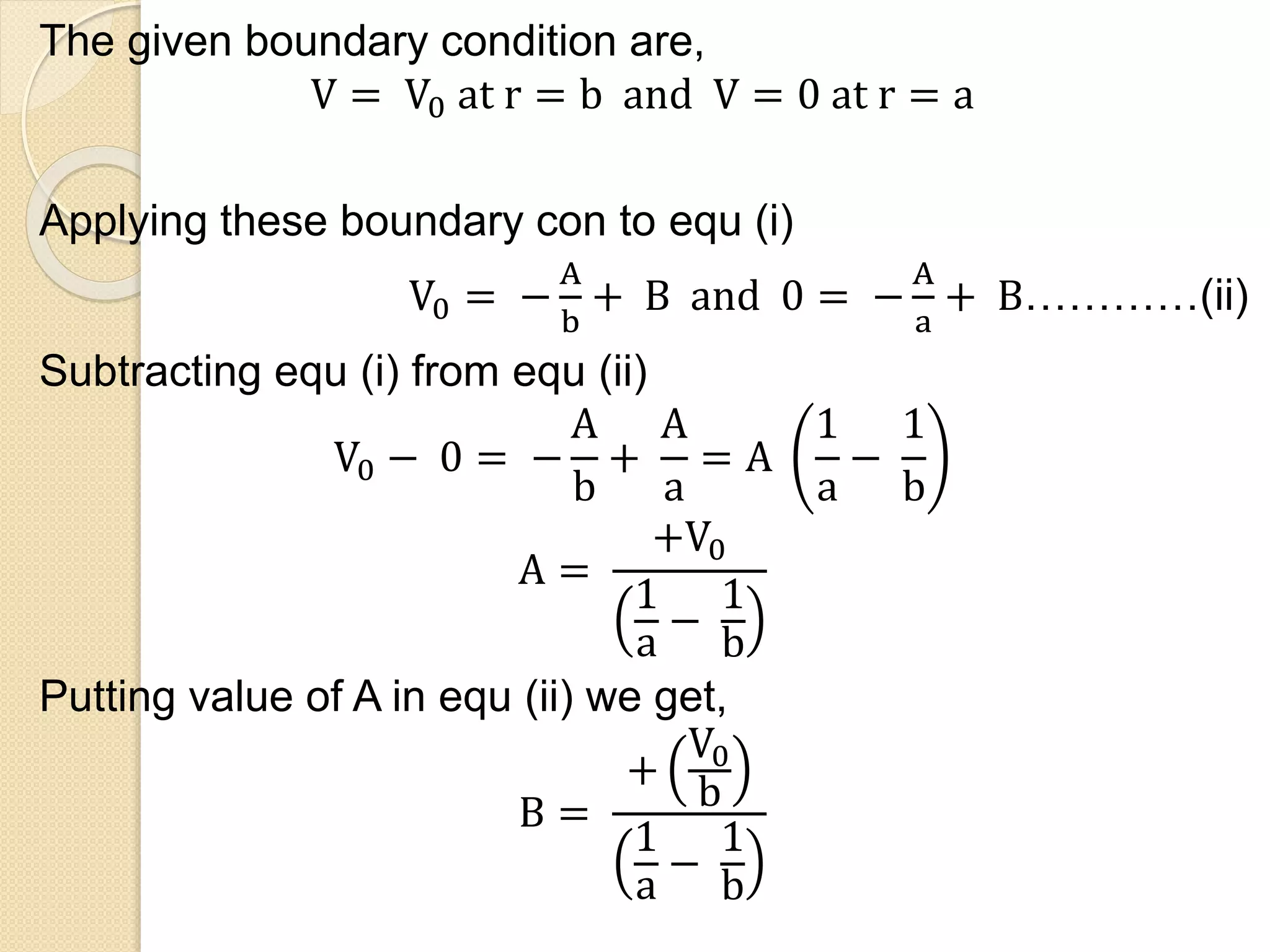
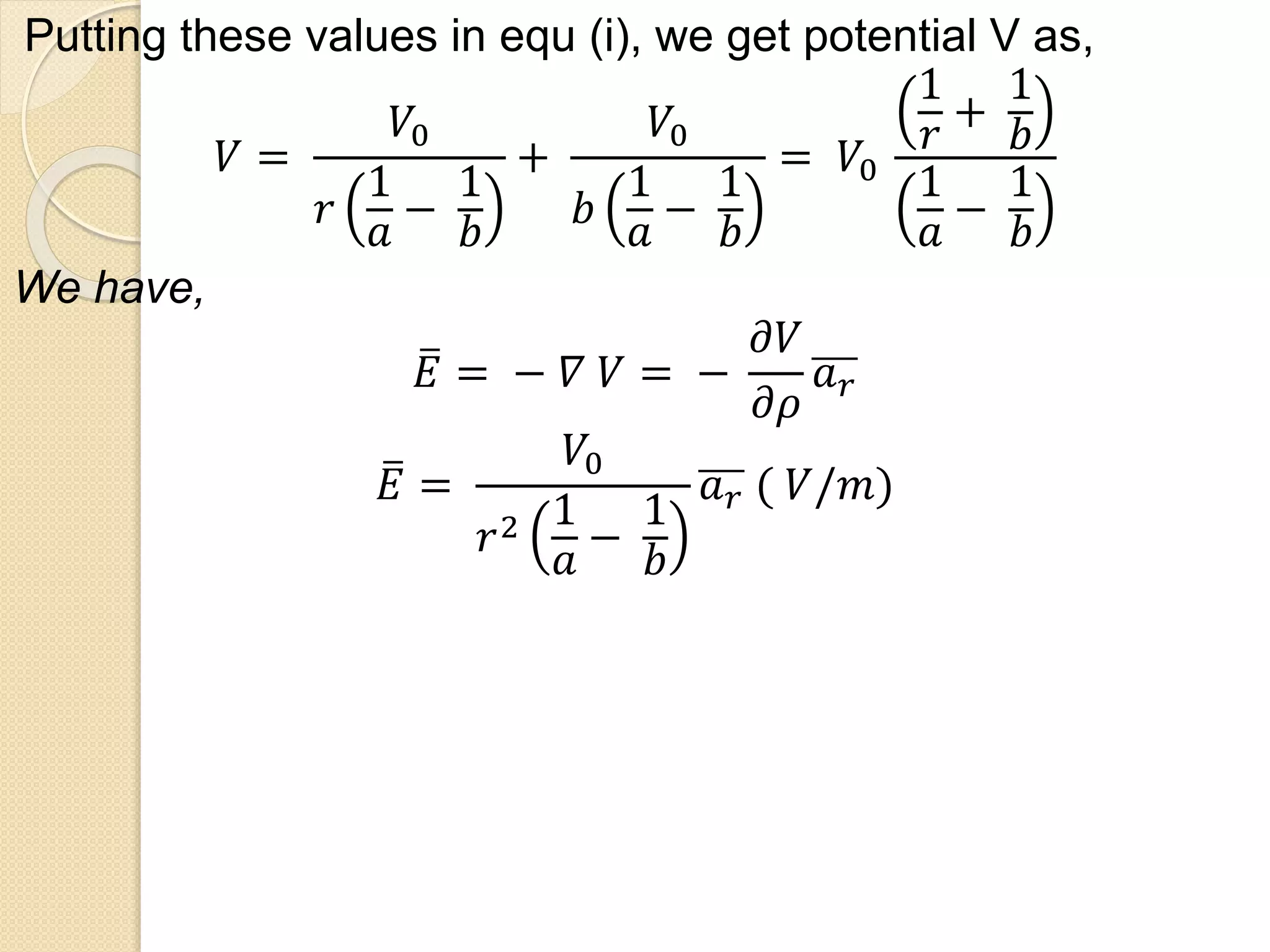
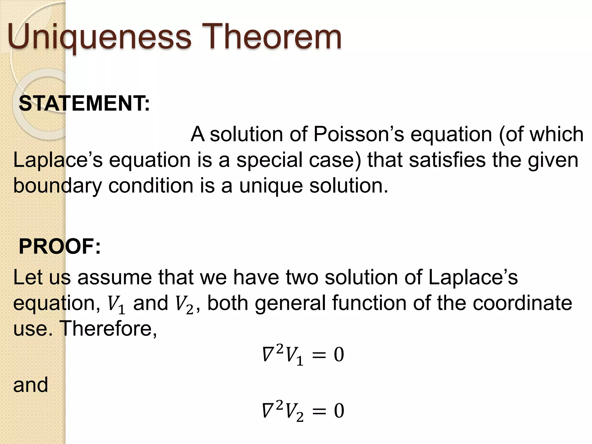
This document discusses Poisson's and Laplace's equations in the context of a class on field theory taught by Prof. Supraja. It provides definitions and derivations of Poisson's and Laplace's equations in different coordinate systems. It gives examples of using these equations to find electric potential and field between charged surfaces, as well as the capacitance between them. It also states the uniqueness theorem, which guarantees a unique solution to Laplace's/Poisson's equation given the boundary conditions.

1. Gandhinagar Institute
Of Technology
Subject – Field Theory (2140909)
Branch – Electrical
Topic – Poisson’s and Laplace’s Equation

2. Name Enrollment No.
Abhishek Chokshi 140120109005
Himal Desai 140120109008
Dheeraj Yadav 140120109010
Guided By – Prof. Supraja Ma’am

3. Laplace’s and Poisson’s Equation
 We have determined the electric field 𝐸 in a region using
Coulomb’s law or Gauss law when the charge distribution is
specified in the region or using the relation 𝐸 = −𝛻𝑉 when the
potential V is specified throughout the region.
 However, in practical cases, neither the charge distribution nor
the potential distribution is specified only at some boundaries.
These type of problems are known as electrostatic boundary
value problems.
 For these type of problems, the field and the potential V are
determined by using Poisson’s equation or Laplace’s equation.
 Laplace’s equation is the special case of Poisson’s equation.

4.  For the Linear material Poisson’s and Laplace’s equation can
be easily derived from Gauss’s equation
𝛻 ∙ 𝐷 = 𝜌 𝑉
But,
𝐷 =∈ 𝐸
Putting the value of 𝐷 in Gauss Law,
𝛻 ∗ (∈ 𝐸) = 𝜌 𝑉
From homogeneous medium for which ∈ is a constant, we write
𝛻 ∙ 𝐸 =
𝜌 𝑉
∈
Also,
𝐸 = −𝛻𝑉
Then the previous equation becomes,
𝛻 ∙ (−𝛻𝑉) =
𝜌 𝑉
∈
Or,
𝛻 ∙ 𝛻𝑉 = −
𝜌 𝑉
∈

5. 𝛻2
𝑉 = −
𝜌 𝑉
∈
 This equation is known as Poisson’s equation which state that
the potential distribution in a region depend on the local
charge distribution.
 In many boundary value problems, the charge distribution is
involved on the surface of the conductor for which the free
volume charge density is zero, i.e., ƍ=0. In that case, Poisson’s
equation reduces to,
𝛻2 𝑉 = 0
 This equation is known as Laplace’s equation.

6. Laplace Equation in Three Coordinate
System
 In Cartesian coordinates:
𝛻𝑉 =
𝜕𝑉
𝜕𝑥
𝑎 𝑥 +
𝜕𝑉
𝜕𝑦
𝑎 𝑦 +
𝜕𝑉
𝜕𝑧
𝑎 𝑧
and,
𝛻𝐴 =
𝜕𝐴 𝑥
𝜕𝑥
+
𝜕𝐴 𝑦
𝜕𝑦
+
𝜕𝐴 𝑧
𝜕𝑧
Knowing
𝛻2
𝑉 = 𝛻 ∙ 𝛻𝑉
Hence, Laplace’s equation is,
𝛻2 𝑉 =
𝜕2 𝑉
𝜕𝑥2 +
𝜕2 𝑉
𝜕𝑦2 +
𝜕2 𝑉
𝜕𝑧2 = 0

7.  In cylindrical coordinates:
𝛻 ∙ 𝑉 =
𝜕𝑉
𝜕𝜌
𝑎 𝜌 +
1
𝜌
𝜕𝑉
𝜕∅
𝑎∅ +
𝜕𝑉
𝜕𝑧
𝑎 𝑧
and,
𝛻 ∙ 𝐴 =
1
𝜌
𝜕
𝜕𝜌
(𝜌𝐴 𝜌) +
1
𝜌
𝜕𝐴∅
𝜕∅
+
𝜕𝐴 𝑧
𝜕𝑧
Knowing
𝛻2
𝑉 = 𝛻 ∙ 𝛻𝑉
Hence, Laplace’s equation is,
𝛻2
𝑉 =
1
𝜌
𝜕
𝜕𝜌
(𝜌
𝜕𝑉
𝜕𝜌
) +
1
𝜌2
𝜕2 𝑉
𝜕∅2 +
𝜕2 𝑉
𝜕𝑧2 = 0

8.  In spherical coordinates:
𝛻 ∙ 𝑉 =
𝜕𝑉
𝜕𝑟
𝑎 𝑟 +
1
𝑟
𝜕𝑉
𝜕𝜃
𝑎 𝜃 +
1
𝑟 sin 𝜃
𝜕𝑉
𝜕∅
𝑎∅
and,
𝛻 ∙ 𝐴 =
1
𝑟2
𝜕
𝜕𝑟
(𝑟2
𝐴 𝑟) +
1
𝑟 sin 𝜃
𝜕
𝜕𝜃
(𝐴 𝜃 sin 𝜃) +
1
𝑟 sin 𝜃
𝜕𝐴∅
𝜕∅
Knowing
𝛻2
𝑉 = 𝛻 ∙ 𝛻𝑉
Hence, Laplace’s equation is,
𝛻2
𝑉 =
1
𝑟2
𝜕
𝜕𝑟
(𝑟2
𝜕𝑉
𝜕𝑟
) +
1
𝑟2 sin 𝜃
𝜕
𝜕𝜃
(sin 𝜃
𝜕𝑉
𝜕𝜃
) +
1
𝑟2 sin 𝜃
𝜕2
𝑉
𝜕∅2
= 0

9. Application of Laplace’s and Poisson’s
Equation
 Using Laplace or Poisson’s equation we can obtain:
1. Potential at any point in between two surface when
potential at two surface are given.
2. We can also obtain capacitance between these two
surface.

10. EXAMPLE:
Let 𝑉 = 2𝑥𝑦3
𝑧3
and ∈=∈0. Given point P(1,3,-1).Find V at
point P. Also Find V satisfies Laplace equation.
SOLUTION:
𝑉 = 2𝑥𝑦3
𝑧3
V(1,3,-1) = 2*1*32(−1)3
= -18 volt
Laplace equation in Cartesian system is
𝛻2 𝑉 =
𝜕2 𝑉
𝜕𝑥2 +
𝜕2 𝑉
𝜕𝑦2 +
𝜕2 𝑉
𝜕𝑧2 = 0
Differentiating given V,
𝜕𝑉
𝜕𝑥
= 2𝑦2
𝑧3 𝜕2 𝑉
𝜕𝑥2 = 0

11. 𝜕𝑉
𝜕𝑦
= 4𝑥𝑦𝑧3 𝜕2 𝑉
𝜕𝑦2 = 4𝑥𝑧3
𝜕𝑉
𝜕𝑧
= 6𝑥𝑦2 𝑧2 𝜕2 𝑉
𝜕𝑧2 = 12𝑥𝑦2 𝑧
Adding double differentiating terms,
𝜕2 𝑉
𝜕𝑥2 +
𝜕2 𝑉
𝜕𝑦2 +
𝜕2 𝑉
𝜕𝑧2 = 0 + 4*𝑧2
+ 12*x*𝑦2
*z ≠ 0
Thus given V does not satisfy Laplace equation

12. EXAMPLE:
 Consider two concentric spheres of radii a and b, a<b. The
outer sphere is kept at a potential 𝑉0 and the inner sphere at
zero potential. Solve Laplace equation in spherical
coordinates to find,
1. The potential and electric field in the region between two
spheres.
2. Find the capacitance between them.
SOLUTION:
From the given data it is clear that V is a function of r only.
i.e.
𝜕𝑉
𝜕𝜃
and
𝜕𝑉
𝜕𝜙
are zero. We know the Laplace's equation in
spherical coordinate system as,
𝛻2
𝑉 =
1
r2
𝜕
𝜕𝑟
𝑟2
𝜕𝑉
𝜕𝑟
+
1
𝑟2 sin 𝜃
𝜕
𝜕𝜃
sin 𝜃
𝜕𝑉
𝜕𝜃
+
1
𝑟2 sin 𝜃
𝜕2 𝑉
𝜕𝜙2
= 0

13. This equation reduces to,
𝛻2 𝑉 =
1
r2
𝜕
𝜕𝑟
𝑟2
𝜕𝑉
𝜕𝑟
= 0
𝑖. 𝑒.
𝜕
𝜕𝑟
𝑟2
𝜕𝑉
𝜕𝑟
= 0
By Integrating we get,
𝑟2
𝜕𝑉
𝜕𝑟
= 𝐴
Or,
𝜕𝑉
𝜕𝑟
=
𝐴
𝑟2
Integrating again we get,
𝑉 = −
𝐴
𝑟
+ 𝐵…………………(i)

14. The given boundary condition are,
V = V0 at r = b and V = 0 at r = a
Applying these boundary con to equ (i)
V0 = −
A
b
+ B and 0 = −
A
a
+ B…………(ii)
Subtracting equ (i) from equ (ii)
V0 − 0 = −
A
b
+
A
a
= A
1
a
−
1
b
A =
+V0
1
a
−
1
b
Putting value of A in equ (ii) we get,
B =
+
V0
b
1
a
−
1
b

15. Putting these values in equ (i), we get potential V as,
𝑉 =
𝑉0
𝑟
1
𝑎
−
1
𝑏
+
𝑉0
𝑏
1
𝑎
−
1
𝑏
= 𝑉0
1
𝑟
+
1
𝑏
1
𝑎
−
1
𝑏
We have,
𝐸 = − 𝛻 𝑉 = −
𝜕𝑉
𝜕𝜌
𝑎 𝑟
𝐸 =
𝑉0
𝑟2 1
𝑎
−
1
𝑏
𝑎 𝑟 ( 𝑉/𝑚)

16. (b) To Find capacitance :
The flux density is,
𝐷 = ∈ 𝐸 =
∈ 𝑉0
𝑟2 1
𝑎
−
1
𝑏
𝑎 𝑟 (𝐶/𝑚2
)
The charge density on the inner sphere i.e. at r=a is,
𝜌𝑠 = 𝐷 | 𝑟 = 𝑎 ∙ 𝑎 𝑟 =
∈ 𝑉0
𝑎2 1
𝑎
−
1
𝑏
(𝐶/𝑚2
)
The capacitance is now calculated by,
𝐶 =
𝑄
𝑉0
=
4 𝜋 𝑎2 𝜌 𝑠
𝑉0
=
4𝜋∈
1
𝑎
−
1
𝑏
(𝐹)…...Ans

17. EXAMPLES:
 Two parallel conducting disks are separated by a distance
5mm at Z=0 and Z=5 mm. If V=0 at Z=0 and V=100 at
z=5 mm. Find charge densities on the disks.
SOLUTION:
From the given con. It is clear that V is a fun. Of z only.
Laplace’s equation of cylindrical coordinate system, we get
𝛻2
𝑉 =
𝜕2
V
𝜕z2
= 0; 𝑖. 𝑒
𝜕2
V
𝜕z2
= 0
Integrating twice we get,
dV
d2
= A and V = Az + B … … i

18. Where, A and B are constants of integration. To determine
these constants apply the boundary conditions.
V=0 at z=0 and V=100 Volts at z=5 mm
Putting these in equ (i)
0 = 𝐴 0 + 𝐵 𝑎𝑛𝑑 100 = 𝐴 5 × 10−3
+ 𝐵
𝐵 = 0 𝑖. 𝑒. 𝐴 =
100
5 × 10−3
= 20 × 103
Putting these in equ (i), the potential is obtained as,
𝑉 = 20 × 103 𝑧
Now, the electric field between the circular disks is obtained
using the relation,
𝐸 = − 𝛻 𝑉 = −
𝜕𝑉
𝜕𝜌
𝑎 𝜌 +
𝜕𝑉
𝜌 𝜕∅
𝑎∅ +
𝜕𝑉
𝜕𝑧
𝑎 𝑧

19. E = −
𝜕V
𝜕z
az = − 20 × 103
az
consider, the medium between the circular disks as free
space, which gives the flux density as,
D = ∈0 E =
10−9
36 π
× −20 × 103
az
= −0.177 × 10−6
az (C /m2
)
Since D is constant between the phase and normal to the
plates, we say that
ρs = Dn = ±0.177 × 10−6
az (C /m2
)

20. Uniqueness Theorem
STATEMENT:
A solution of Poisson’s equation (of which
Laplace’s equation is a special case) that satisfies the given
boundary condition is a unique solution.
PROOF:
Let us assume that we have two solution of Laplace’s
equation, 𝑉1 and 𝑉2, both general function of the coordinate
use. Therefore,
𝛻2 𝑉1 = 0
and
𝛻2 𝑉2 = 0

21. Also assume that both 𝑉1 and 𝑉2 satisfies the same
boundary condition . Let us define a new difference
potential :
𝑉1 − 𝑉2 = 𝑉𝑑
Now
𝛻2(𝑉1 − 𝑉2) = 0
i.e
𝛻2
𝑉𝑑 = 0
We have the vector identity,
𝛻 ∙ 𝑉𝐷 = 𝑉 𝛻 ∙ 𝐷 + 𝐷 ∙ (𝛻𝑉)
Let V= 𝑉𝑑 and D= 𝛻 𝑉𝑑 , then we have
𝛻 ∙ 𝑉𝑑 𝛻 𝑉𝑑 = 𝑉𝑑 𝛻2 𝑉𝑑 + 𝛻𝑉𝑑
2
From the above equation, 𝛻2
𝑉𝑑 = 0, then we have
𝛻 ∙ 𝑉𝑑 𝛻 𝑉𝑑 = 𝛻𝑉𝑑
2

22. Taking the volume integral over the volume gives,
𝑉
𝛻 ∙ 𝑉𝑑 𝛻 𝑉𝑑 𝑑𝑣 =
𝑣
𝛻𝑉𝑑
2
𝑑𝑣
Now the divergent theorem is:
𝑠
𝐷𝑑 𝑠 =
𝑣
(𝛻 ∙ 𝐷)𝑑𝑣
The right hand side of above equation can now be written in
term of surface integral as,
𝑠
𝑉𝑑 𝛻 𝑉𝑑 ∙ 𝑑 𝑠 =
𝑣
𝛻𝑉𝑑
2 𝑑𝑣
 The surface integral can be evaluated by considering the
surface of very large sphere with radius R. when R is very
large both 𝑉1 and 𝑉2 can be treated as a point charge,
since size of it will be very small compared to R. Hence
the surface integral on LHS decreases and approaches

23. 𝑣
𝛻𝑉𝑑
2
𝑑𝑣 = 0
 Since 𝛻𝑉𝑑
2
is always positive, everywhere above
equation is satisfied only if 𝛻𝑉𝑑=0. If the gradient of 𝑉𝑑 i.e.
𝑉1 − 𝑉2 is everywhere zero, then 𝑉1 − 𝑉2 cannot change
with any coordinates i.e. it has same value at all point on
its boundary surface.
 Therefore, 𝑉1 = 𝑉2 gives two identical solutions, i.e. unique
solution