Downloaded 154 times
![4
SOLO
• Rotation Matrix from Earth to Wind Coordinates
[ ] [ ] [ ]321 χγσ=W
EC
where
σ – Roll Angle
γ – Elevation Angle of the Trajectory
χ – Azimuth Angle of the Trajectory
Force Equation:
amgmTFA
=++
where:
• Aerodynamic Forces (Lift L and Drag D)
( )
−
−
=
L
D
F
W
A 0
• Thrust T ( )
=
α
α
sin
0
cos
T
T
T W
• Gravitation acceleration
( ) ( )
−
−
−
==
g
cs
sc
cs
sc
cs
scgCg EW
E
W
0
0
100
0
0
0
010
0
0
0
001
χχ
χχ
γγ
γγ
σσ
σσ
( )
g
cc
cs
s
g W
−
=
γσ
γσ
γ
α
T
V
L
D
Bx
Wx
Bz
Wz
Wy
By
Flat Earth Three Degrees of Freedom Aircraft Equations](https://image.slidesharecdn.com/12-performanceofanaircraftwithparabolicpolar-sololaptop-150812133215-lva1-app6891/75/12-performance-of-an-aircraft-with-parabolic-polar-4-2048.jpg)
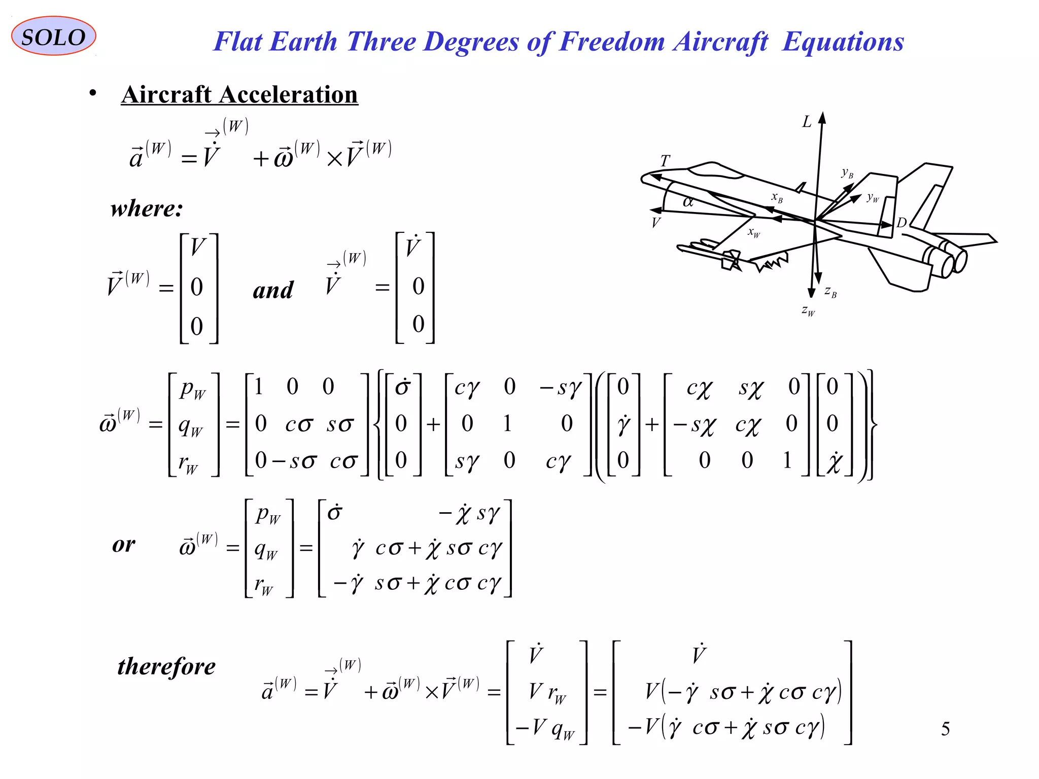
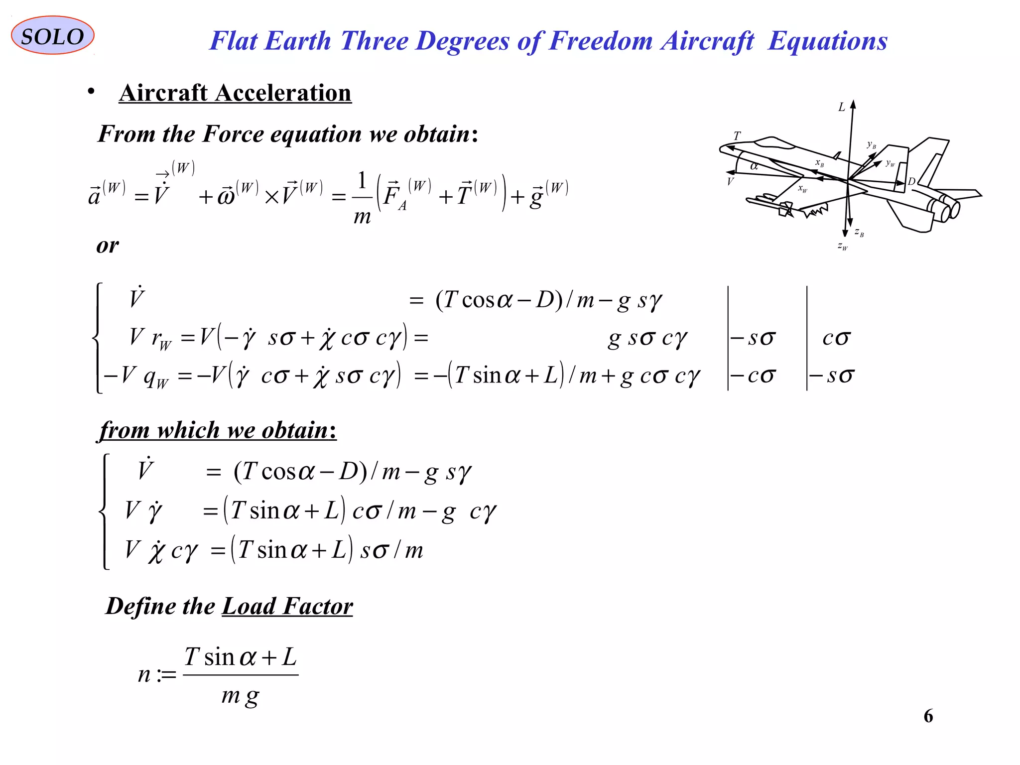
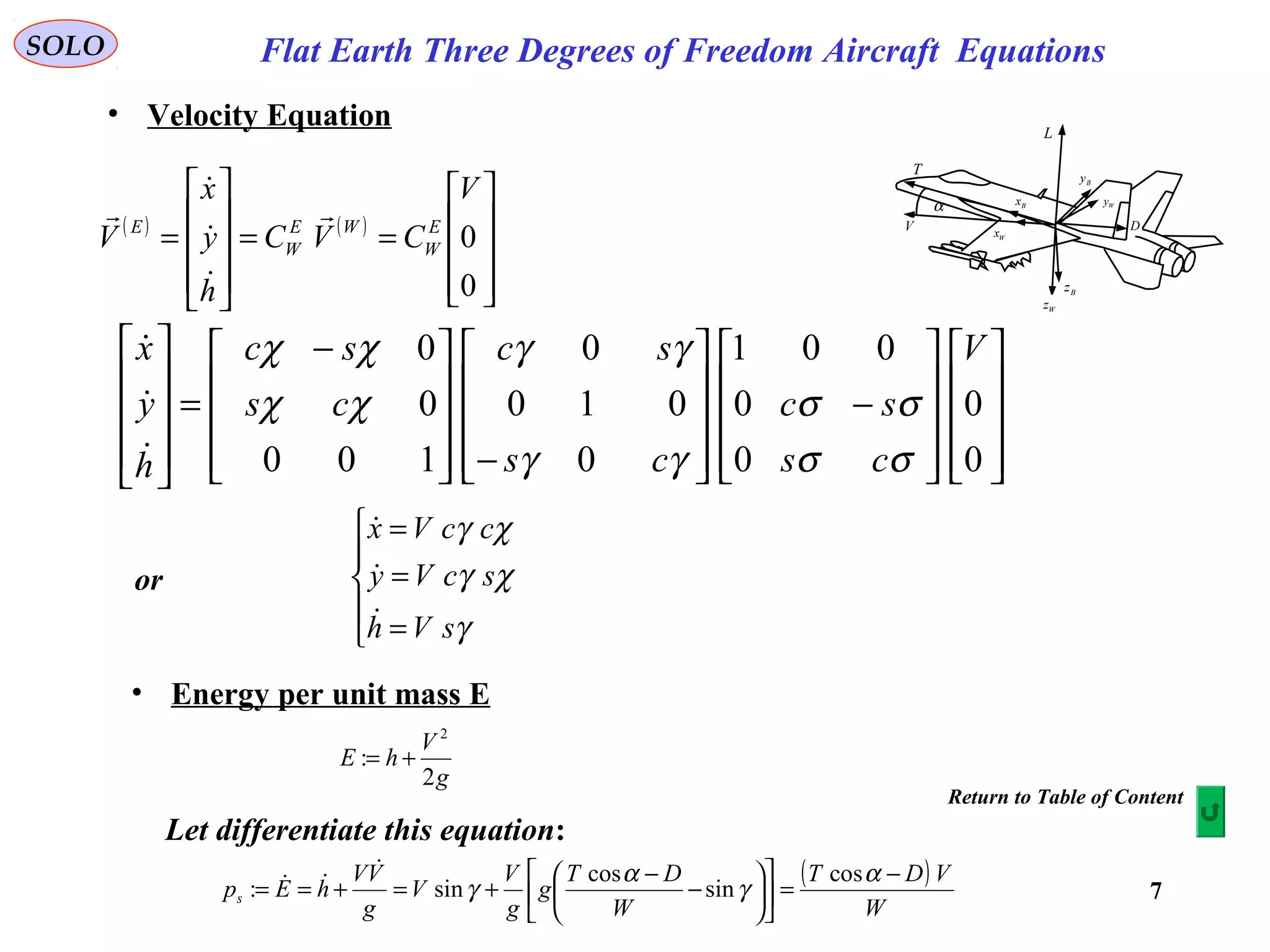
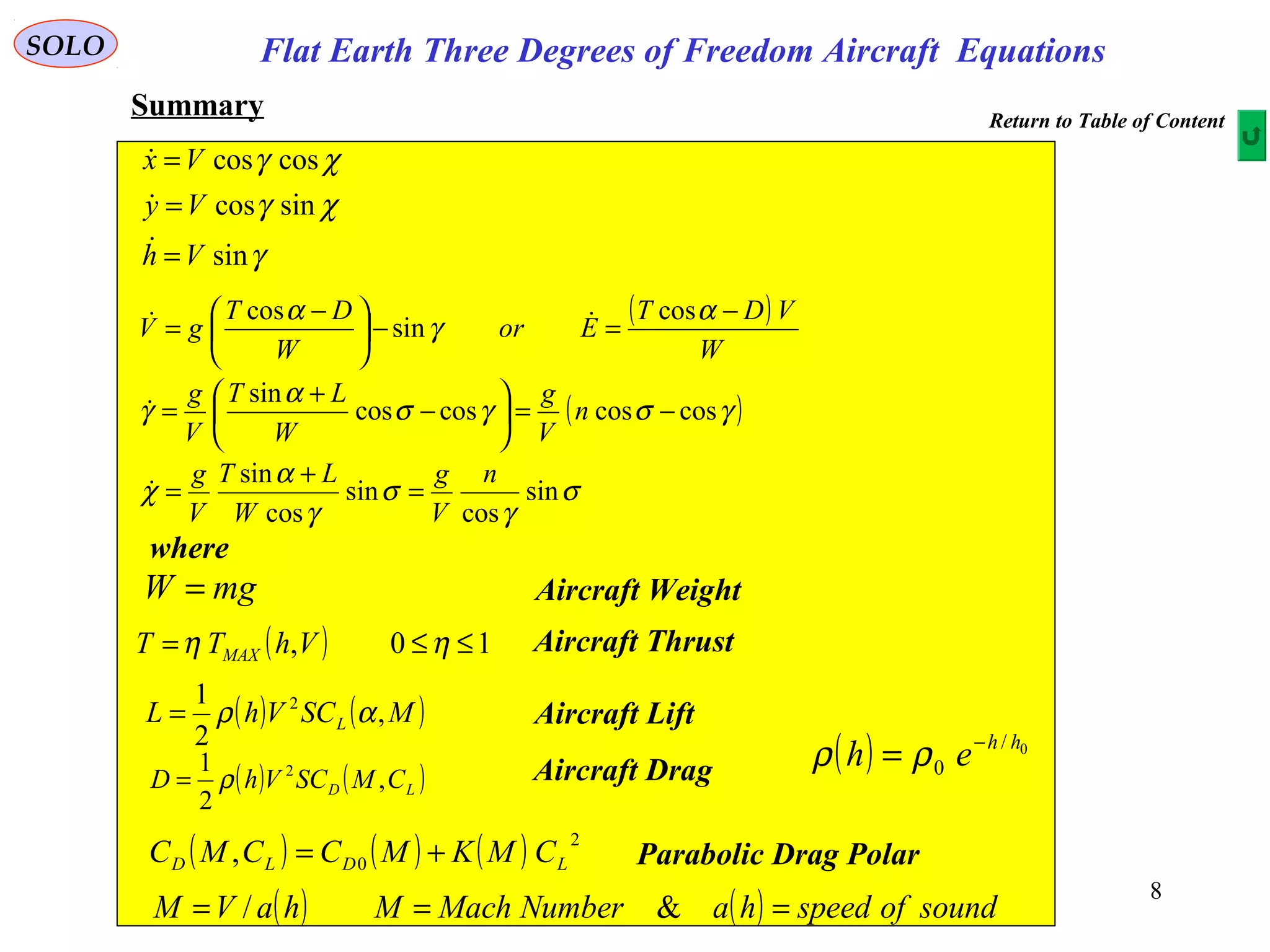
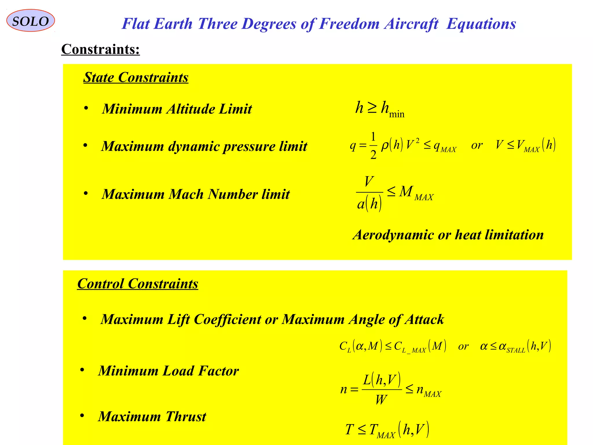
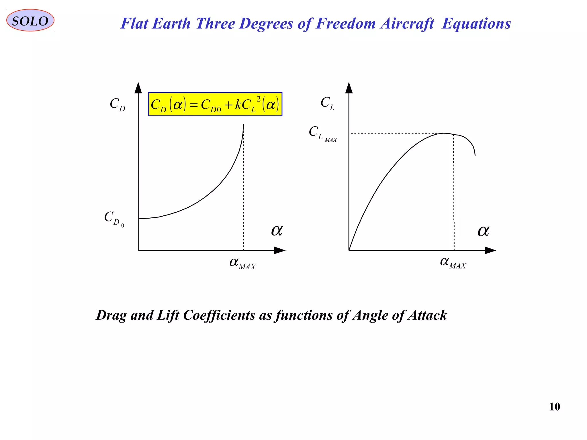
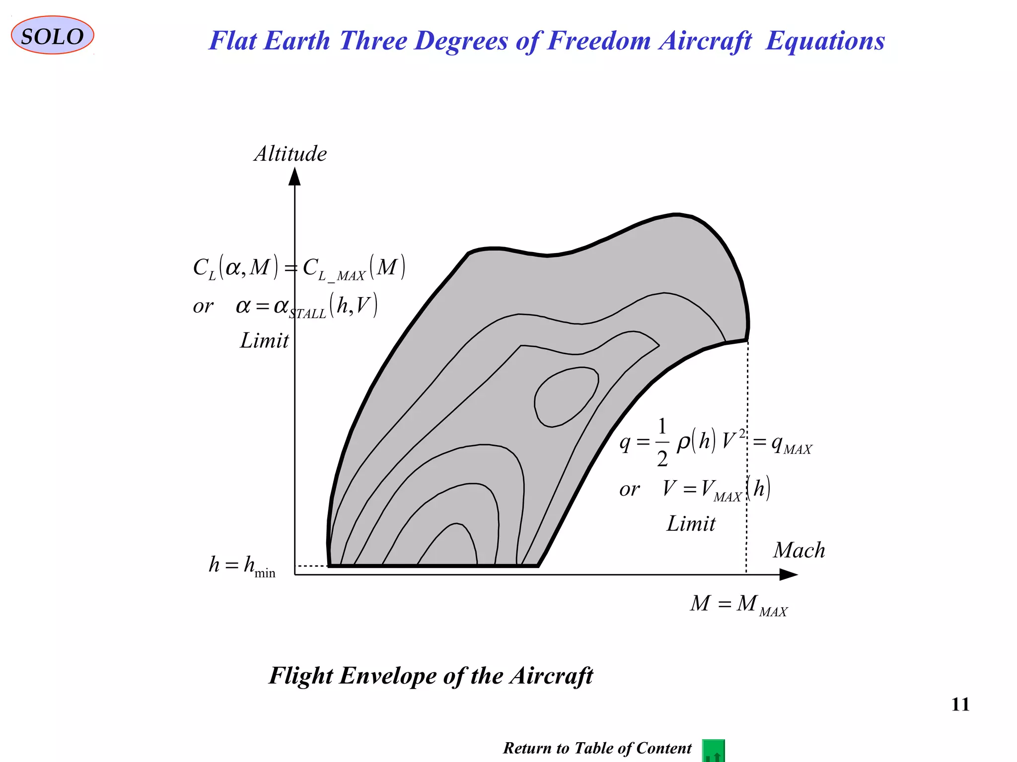
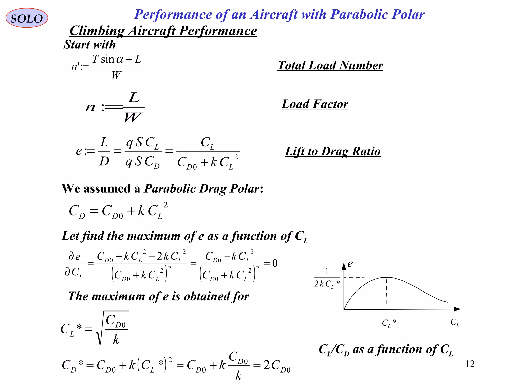
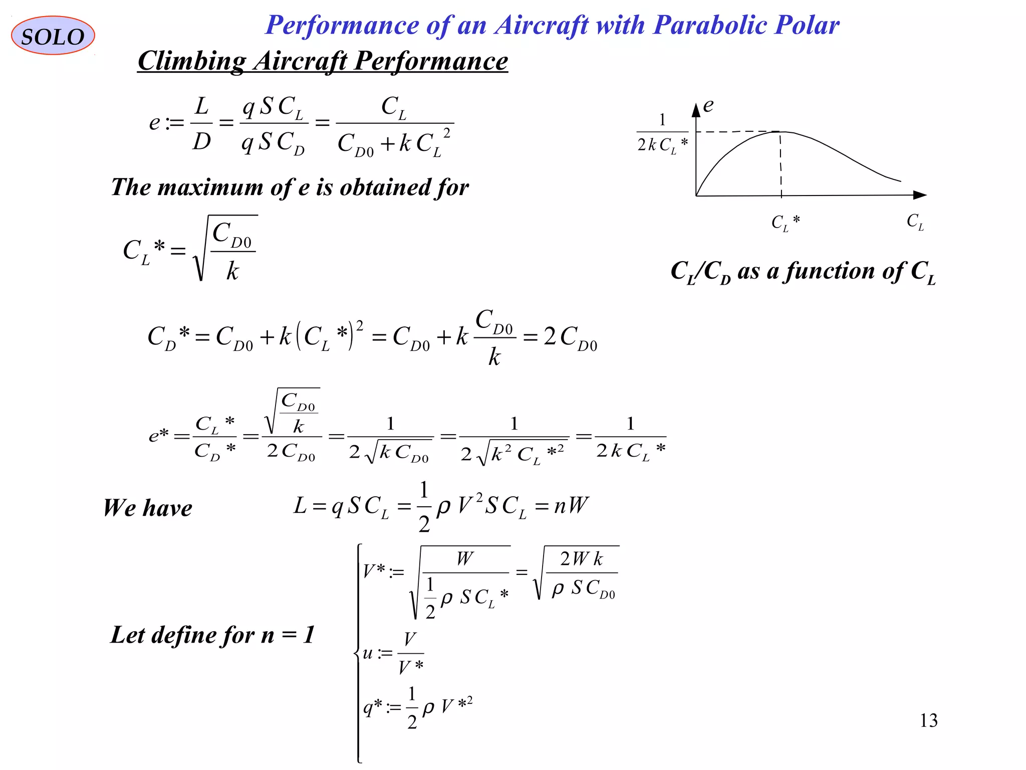
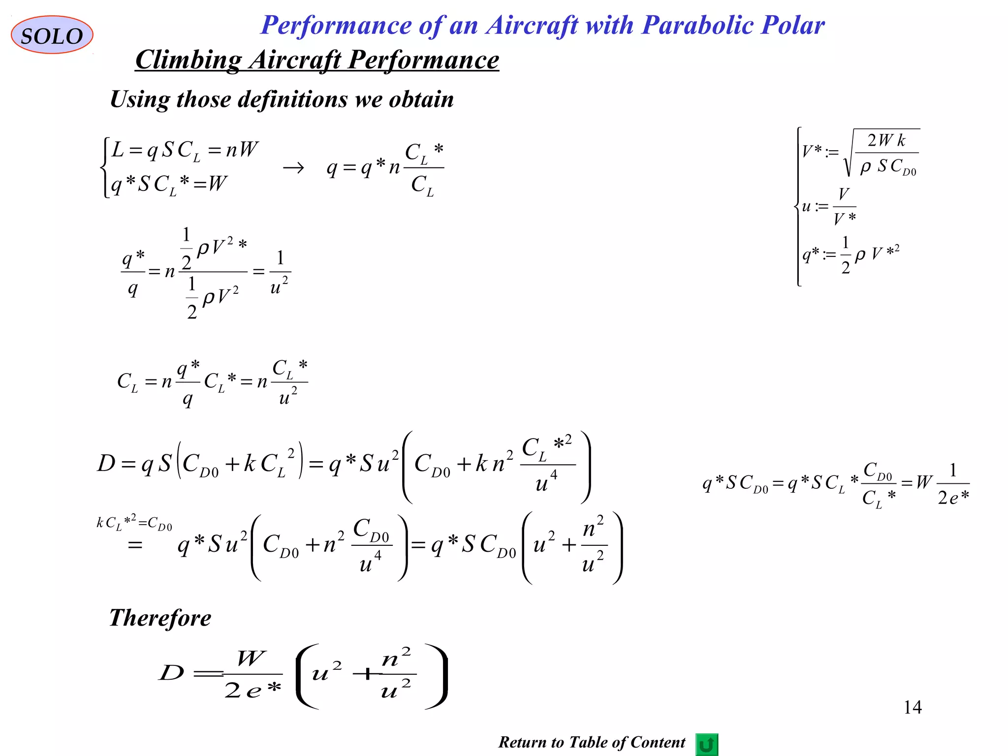
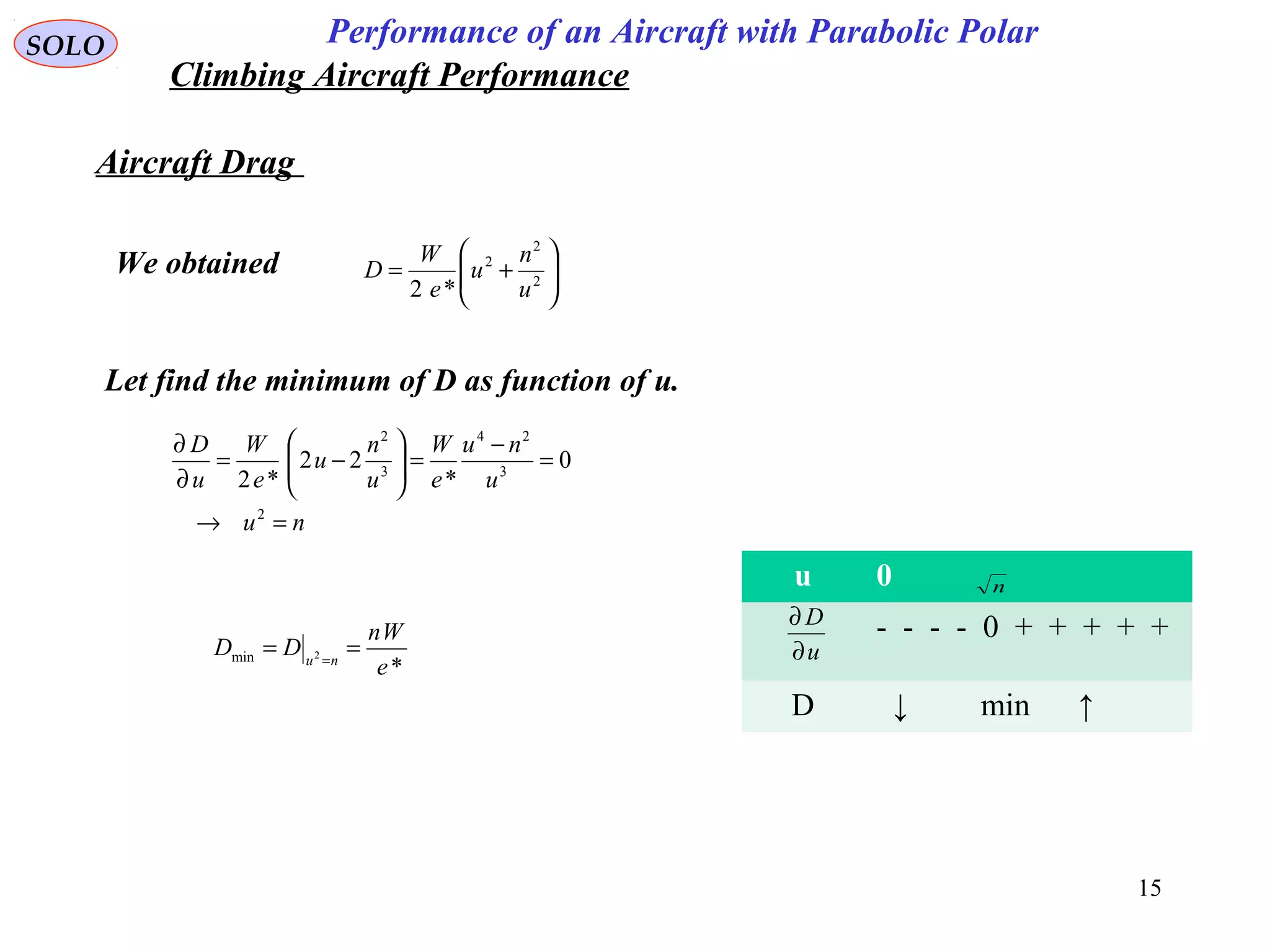
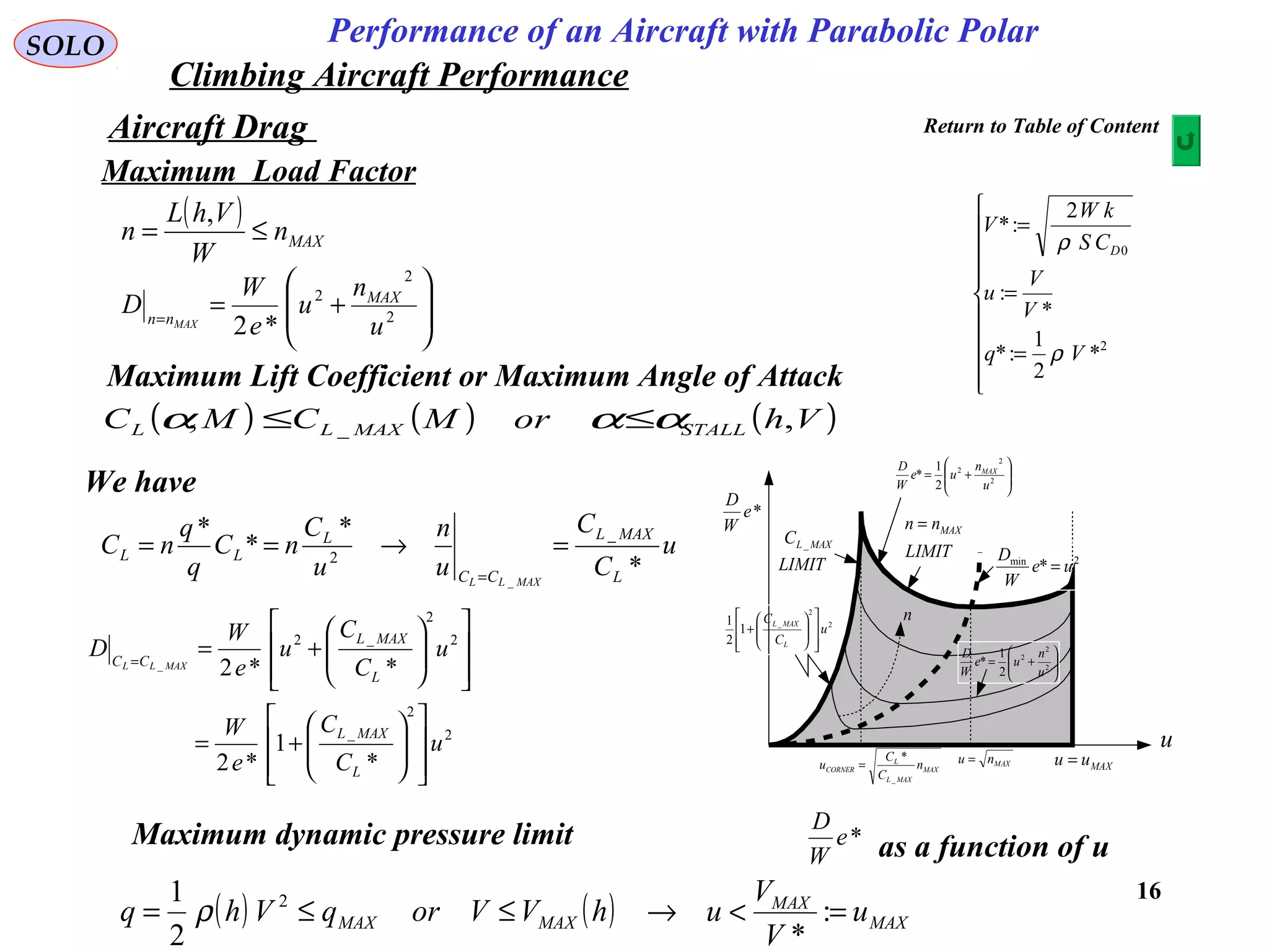
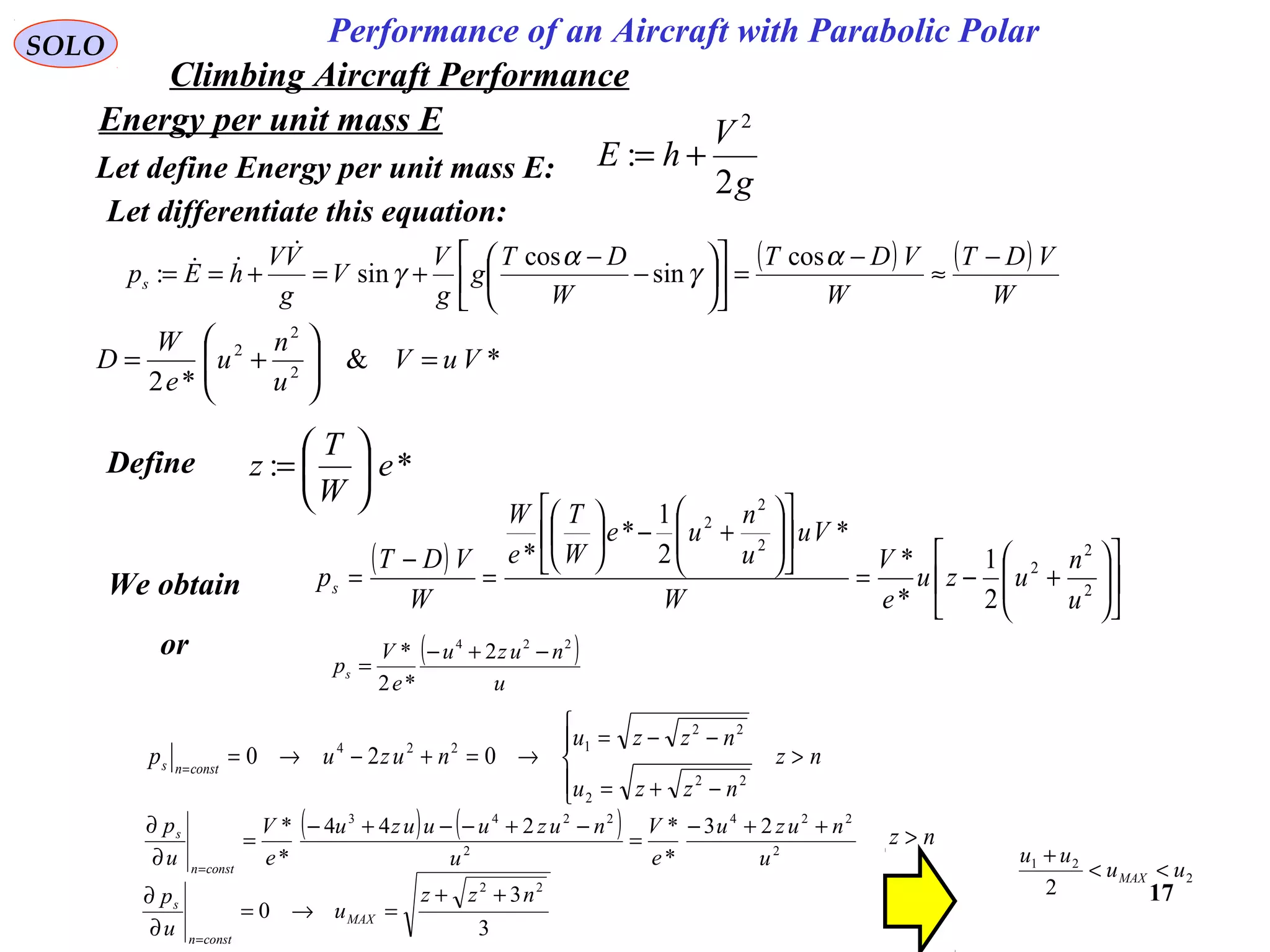
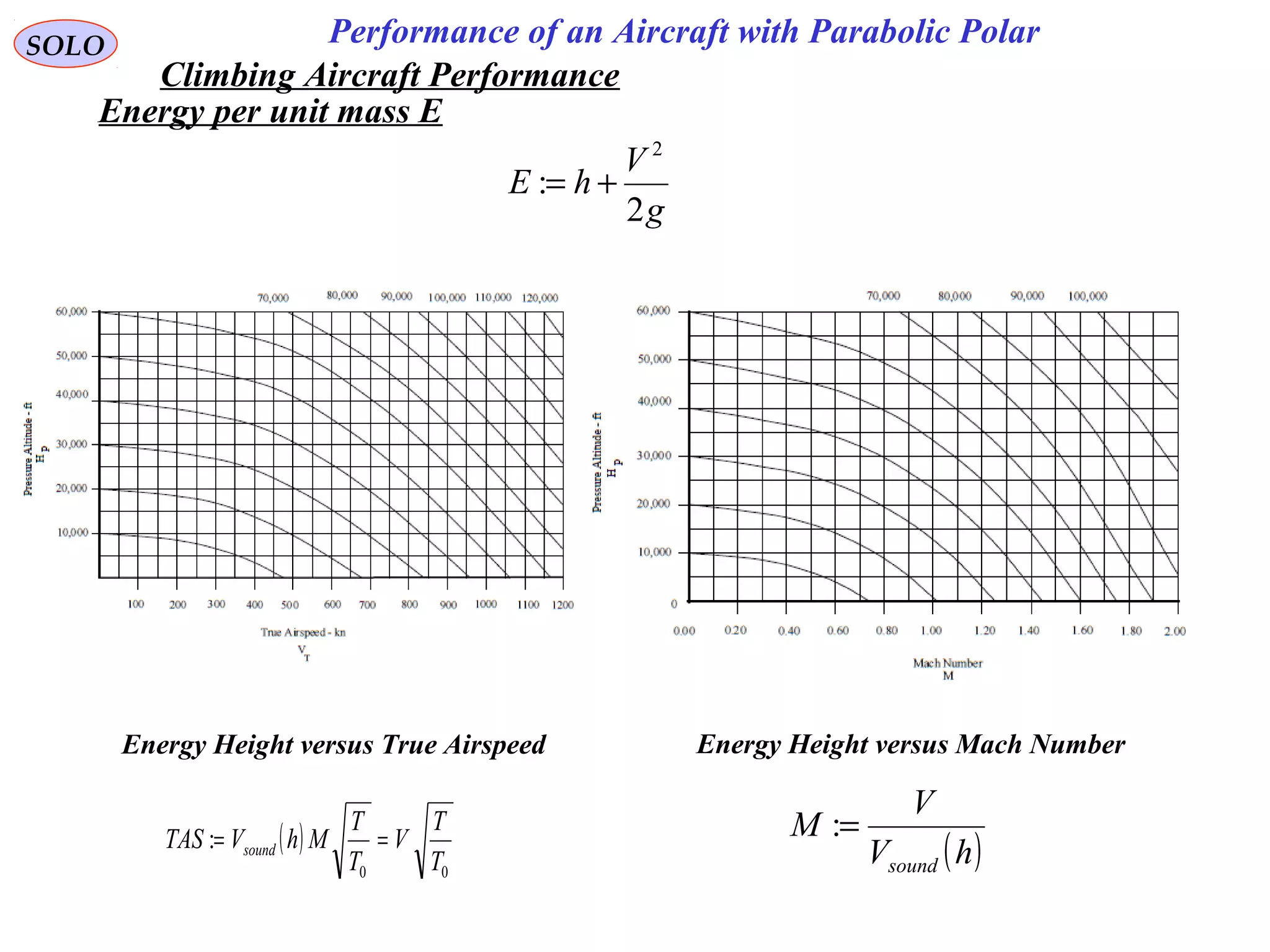
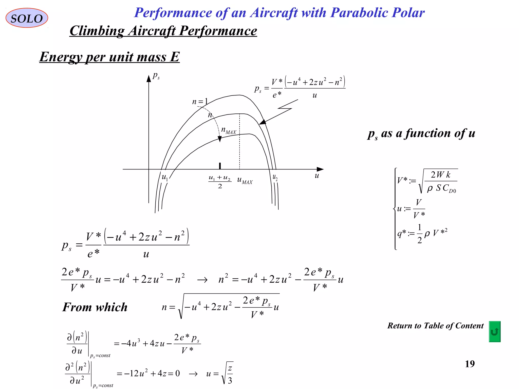
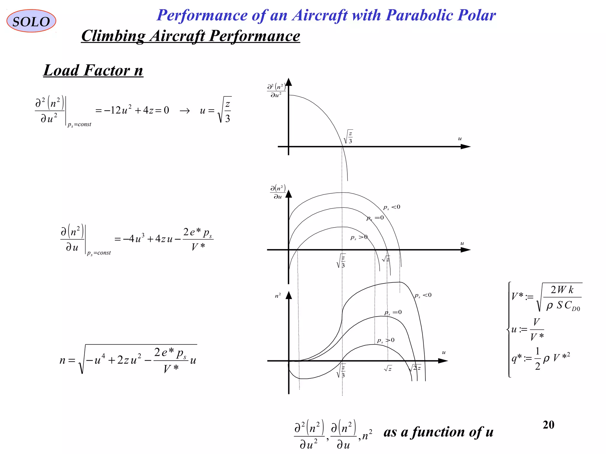


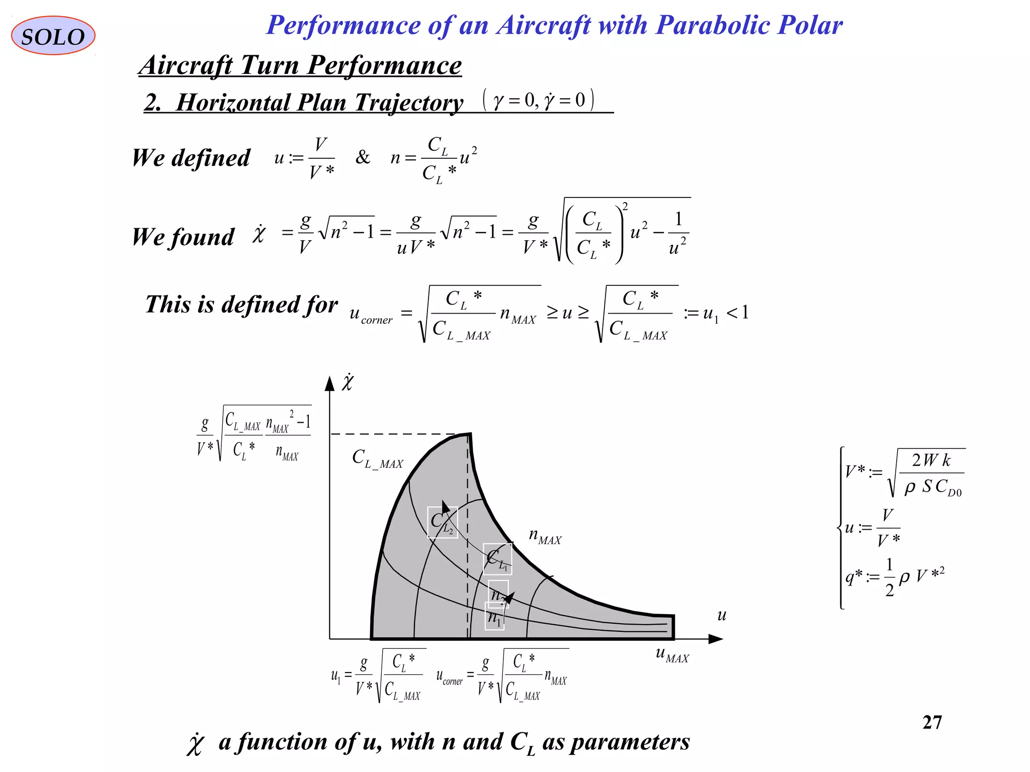


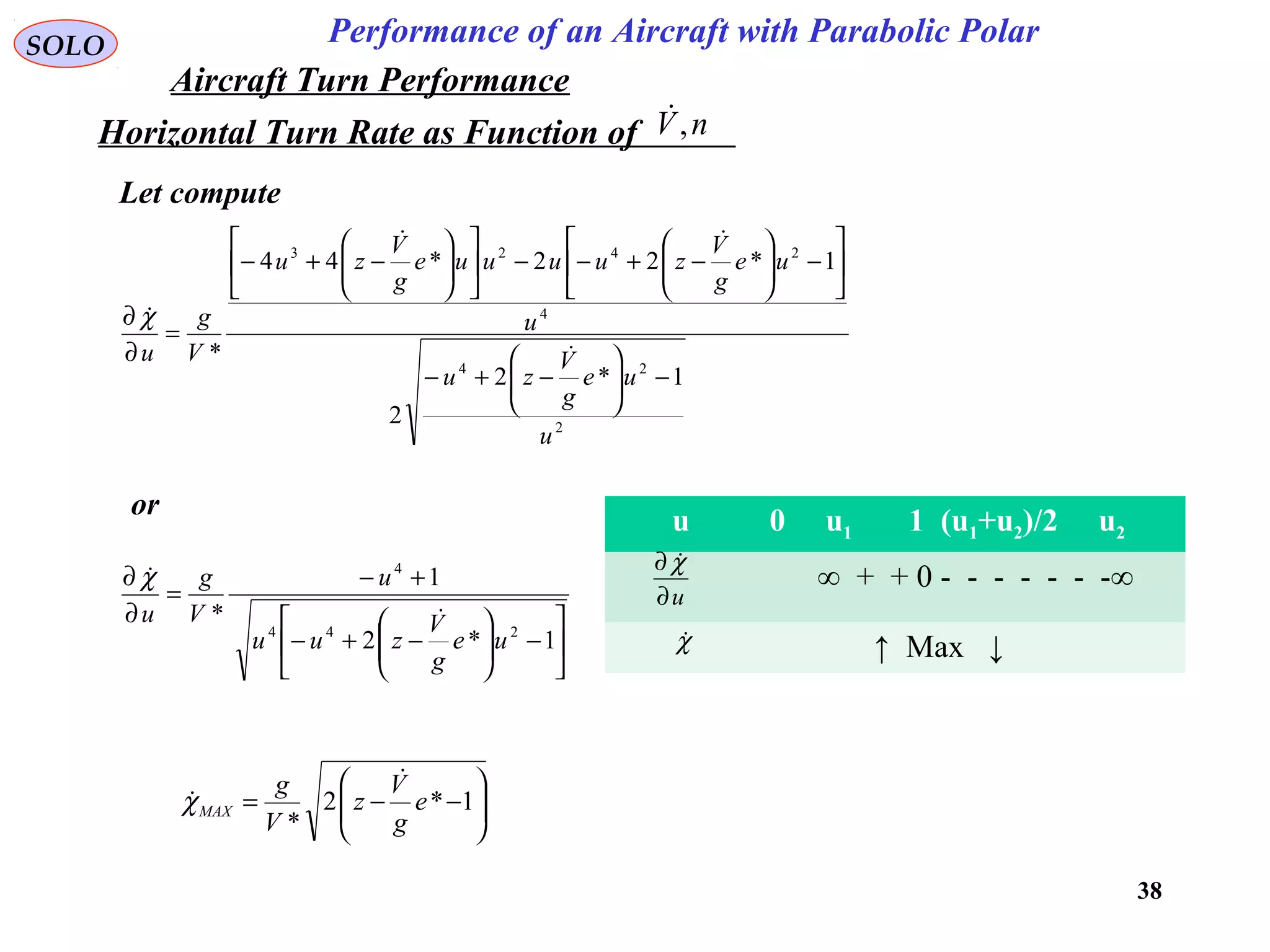
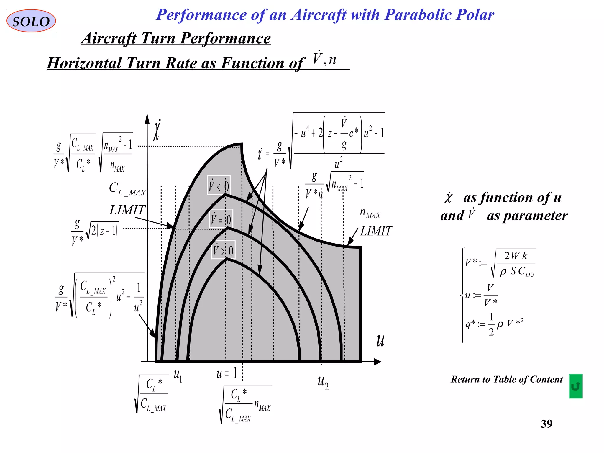

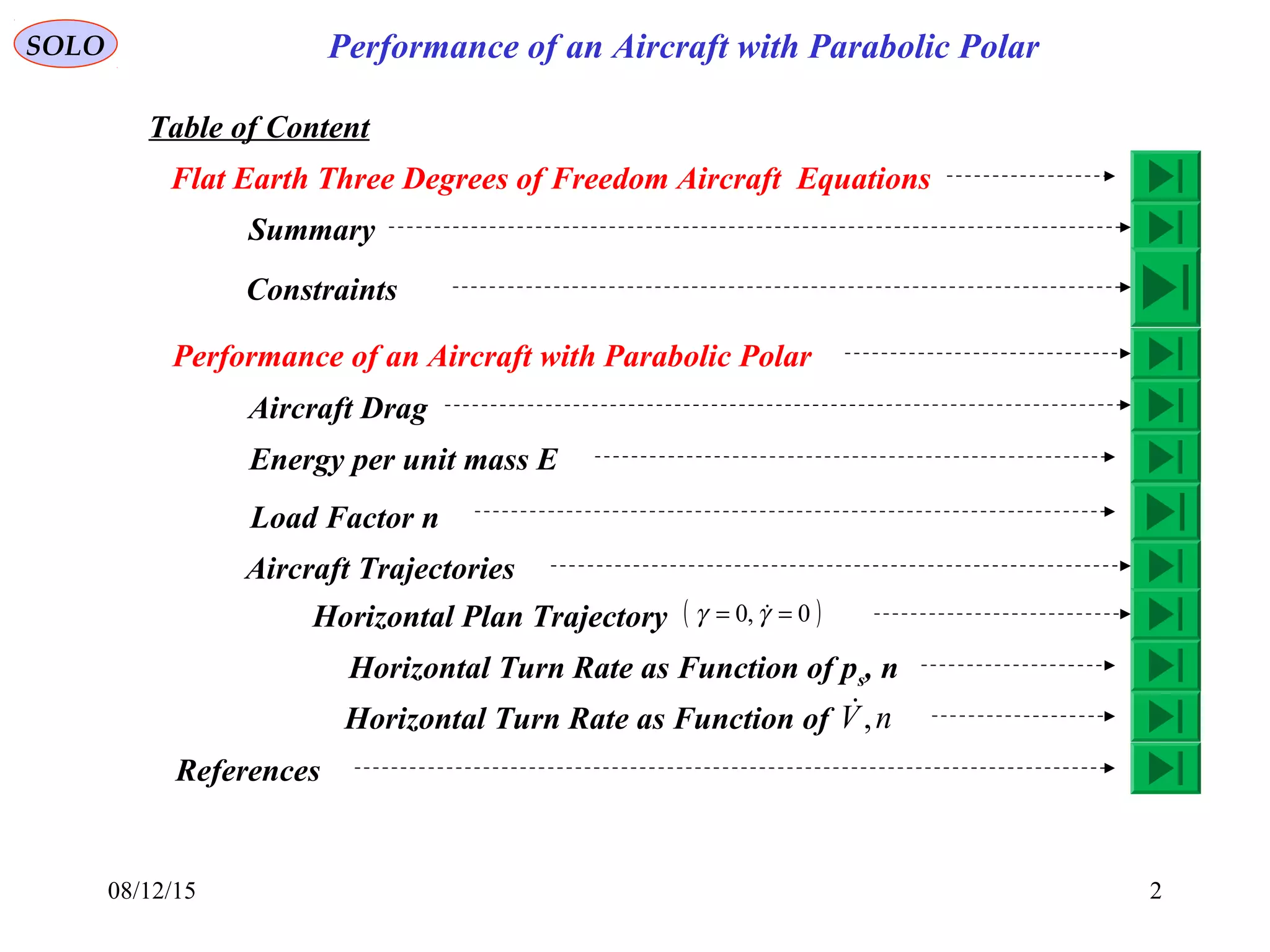
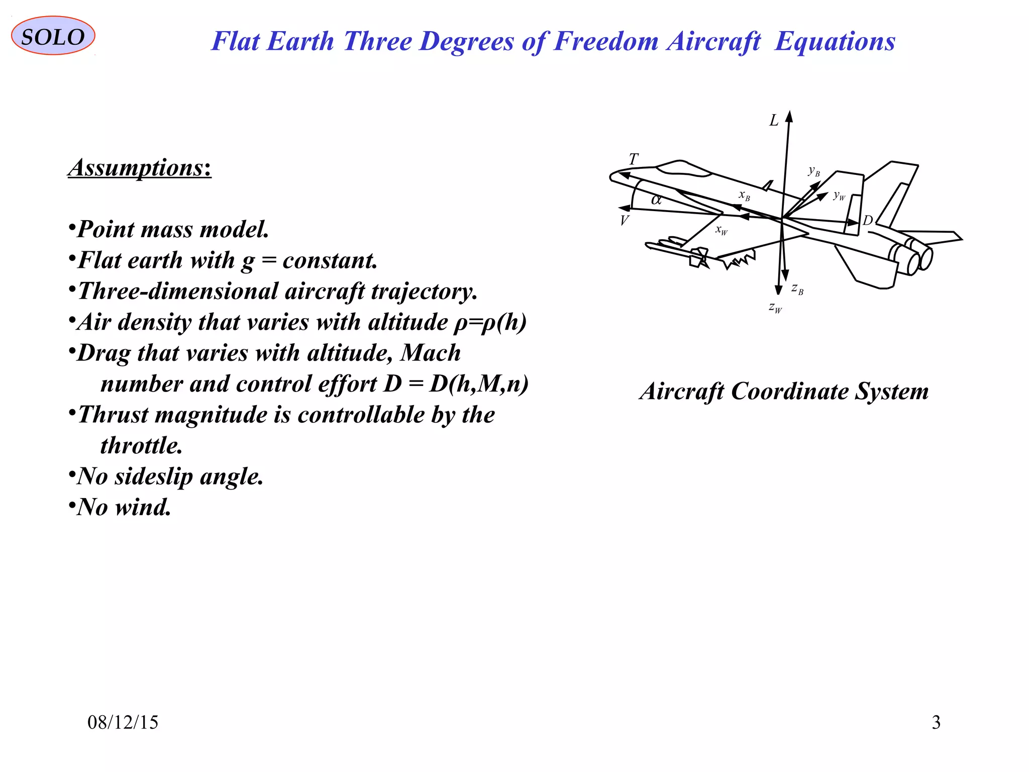
The document discusses the performance of an aircraft modeled with parabolic polar equations, focusing on the forces acting on the aircraft in a flat earth scenario. It includes equations for aerodynamic lift, drag, thrust, and energy per unit mass, while addressing constraints related to altitude, dynamic pressure, and control limits. The analysis emphasizes calculating maximum efficiencies and load factors during different flight trajectories.