Download as PDF, PPTX


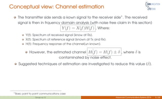

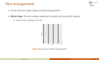
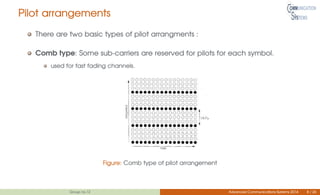


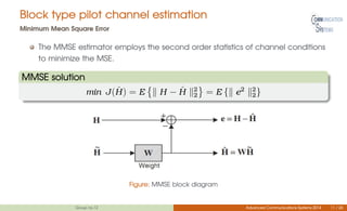


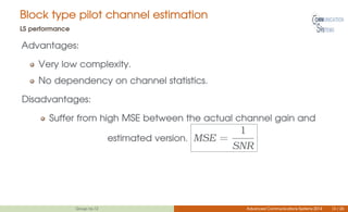


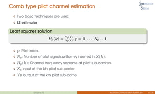
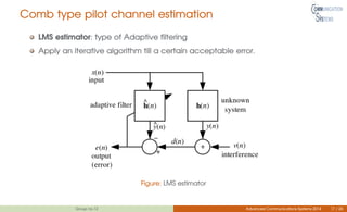
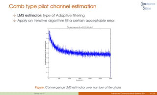


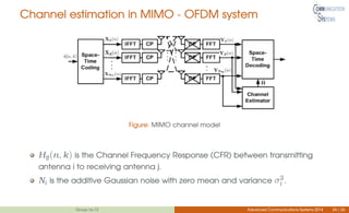


This document discusses channel estimation techniques for OFDM systems. It begins by introducing OFDM and the need for channel state information at the receiver. It then describes two common pilot arrangements - block and comb type. For block pilots, it examines least squares and minimum mean square error channel estimation. It finds MMSE performs better but with higher complexity. For comb pilots, it presents least squares and LMS estimation as well as interpolation techniques between pilot tones. The document also evaluates channel estimation for MIMO-OFDM and the effects of user mobility.