This document summarizes and compares different channel estimation techniques for OFDM systems. It discusses block-type pilot arrangement where pilots are sent on all subcarriers periodically, and comb-type pilot arrangement where pilots are spaced between data symbols. For block-type, channel estimation can be done with LS or MMSE. For comb-type, estimation is done at pilot frequencies using LS, MMSE or LMS, and interpolation between pilots with techniques like linear, cubic spline. Decision feedback equalizer is also implemented for block-type. Performance is evaluated using modulation schemes like QPSK, 16QAM under fading channels, and comb-type is shown to track fast fading better than block-type.

1. International Journal of Research in Advent Technology, Vol.2, No.3, March 2014
E-ISSN: 2321-9637
A Review of Channel Estimation Techniques in
OFDM Systems – Application to PAPR Reduction
122
A Pavani
Asst. Prof., ECE
Priyadarshini College of Engineering
Kamupartipadu, Nellore ,
Andhra Pradesh
Email-ID:Pavani0504@gmail.com
Dr EV Krishna Rao
Professor, ECE
Koneru Lakshmaiah
Educational Foundation (KL
University)
Greenfields, Guntur
Andhra Pradesh
ID: krishnaraoede@yahoo.co.in
Dr B Prabhakara Rao
Rector
JNTUK, Kakinada
Andhra Pradesh
drbprjntu@gmail.com
Abstract- The channel estimation techniques for OFDM systems based on pilot arrangement are investigated. The
channel estimation based on comb type pilot arrangement is studied through different algorithms for both estimating
channel at pilot frequencies and interpolating the channel. The estimation of channel at pilot frequencies is based on
LS and LMS while the channel interpolation is linear interpolation, second order interpolation, low-pass
interpolation, spline cubic interpolation, and time domain interpolation. Time-domain interpolation is obtained by
passing to time domain through IDFT, zero padding and going back to frequency domain through DFT. In addition,
the channel estimation based on block type pilot arrangement is performed by sending pilots at every sub-channel
and using this estimation for a specific number of following symbols. We have also implemented decision feedback
equalizer for all sub-channels followed by periodic block-type pilots. We have compared the performances of all
schemes by measuring bit error rate with 16QAM, QPSK, DQPSK and BPSK as modulation schemes, and multipath
rayleigh fading and AR based fading channels as channel models.
Index Terms: linear interpolation, spline cubic interpolation, 16QAM, QPSK, DQPSK and BPSK
1. INTRODUCTION
Orthogonal Frequency Division Multiplexing
(OFDM) has recently been applied widely in wireless
communication systems due to its high data rate
transmission capability with high bandwidth efficiency
and its robustness to multipath delay. It has been used in
wireless LAN standards such as American IEEE802.11a
and the European equivalent HIPERLAN/2 and in
multimedia wireless services such as Japanese
Multimedia Mobile Access Communications.
A dynamic estimation of channel is necessary
before the demodulation of OFDM signals since the
radio channel is frequency selective and time-variant for
wideband mobile communication systems. The channel
estimation can be performed by either inserting pilot
tones into all of the subcarriers of OFDM symbols with
a specific period or inserting pilot tones into each
OFDM symbol. The first one, block type pilot channel
estimation, has been developed under the assumption of
slow fading channel. Even with decision feedback
equalizer, this assumes that the channel transfer function
is not changing very rapidly. The estimation of the
channel for this block-type pilot arrangement can be
based on LS or MMSE. The MMSE estimate has been
shown to give 10-15 dB gain in SNR for the same mean
square error of channel estimation over LS estimate [1].
In [2], a low-rank approximation is applied to linear
MMSE by using the frequency correlation of the
channel to eliminate the major drawback of MMSE,
which is complexity. The later, the comb-type pilot
channel estimation, has been introduced to satisfy the
need for equalizing the significant changes even in one
OFDM block. The comb-type pilot channel estimation
consists of algorithms to estimate the channel at pilot
frequencies and to interpolate the channel.
The estimation of the channel at the pilot
frequencies for comb-type based channel estimation can
be based on LS, MMSE or LMS. MMSE has been
shown to perform much better than LS. In [3], the
complexity of MMSE is reduced by deriving an optimal
low-rank estimator with singular-value decomposition.
The interpolation of the channel for comb-type
based channel estimation can depend on linear
interpolation, second order interpolation, low-pass
interpolation, spline cubic interpolation, and time
domain interpolation. In [3], second-order interpolation
has been shown to perform better than the linear
interpolation. In [4], time-domain interpolation has been

2. International Journal of Research in Advent Technology, Vol.2, No.3, March 2014
E-ISSN: 2321-9637
123
proven to give lower BER compared to linear
interpolation.
In this paper, our aim is to compare the
performance of all of the above schemes by applying
16QAM, QPSK, DQPSK and BPSK as modulation
schemes, and multipath rayleigh fading and AR based
fading channels as channel models. In section 2, the
description of the OFDM system based on pilot channel
estimation is given. In section 3, the estimation of the
channel based on block-type pilot arrangement is
discussed. In section 4, the estimation of the channel at
pilot frequencies is presented. In section 5, the different
interpolation techniques are introduced. In section 6, the
simulation environment and results are described.
Section 7 concludes the paper.
2. SYSTEM DESCRIPTION
The OFDM system based on pilot channel
estimation is given in Figure 1. The binary information
is first grouped and mapped according to the modulation
in “signal mapper”. After inserting pilots either to all
sub-carriers with a specific period or uniformly between
the information data sequence, IDFT block is used to
transform the data sequence of length N {X(k)} into
time domain signal {x(n)} with the following equation:
1 2
-
N j
( ) { ( )} ( )
kn
x n IDFT X k X k e N
0
= -
0 ,1, 2 , 1 (1 )
= = Σ
k
=
n K
N
p
where N is the DFT length.
Following IDFT block, guard time, which is
chosen to be larger than the expected delay spread, is
inserted to prevent inter-symbol interference. This guard
time includes the cyclically extended part of OFDM
symbol in order to eliminate inter-carrier interference
(ICI). The resultant OFDM symbol is given as follows:
( ) ( )
+ = - - + -
, , 1, , 1
x N n n N N
( ) (2)
x n g g
f L
, 0,1, 1
  
= -
=
x n n N
L
where Ng is the length of the guard interval.
After following D/A converter, this signal will
be sent from the transmitter with the assumption of the
baseband system model. The transmitted signal will
pass through the frequency selective time varying
fading channel with additive noise. The received signal
is given by:
y x (n ) h(n ) w(n ) (3) f f = Ä +
where w(n) is additive white gaussian noise and h(n) is
the channel impulse response, which can be represented
by: [4]
1
r
( ) ( ) 0 1 (4)
Di h n h e d l t
0
2
- £ £ Σ -
=
= - n N
i
i
f Tn
N
j
i
p
where r is the total number of propagation paths, hi is
the complex impulse response of the ith path, fDi is the ith
path Doppler frequency shift, λ is delay spread index, T
is the sample period and ti is the ith path delay
normalized by the sampling time.
At the receiver, after passing to discrete
domain through A/D and low pass filter, guard time is
removed:
y (n ) = y (n + N ) n = 0,1, L
N - 1 (5) f g
Then y(n) is sent to DFT block for the
following operation:
1 1 2
= = - -
( ) { ( )} ( )
Y k DFT y n y n e
N
0
= -
0,1,2, 1 (6)
= Σ
k N
N
kn
N j
n
K
p
Assuming there is no ISI, [7] shows the
relation of the resulting Y(k) to H(k)=DFT{h(n)}, I(k)
that is ICI because of Doppler frequency and
W(k)=DFT{w(n)}, with the following equation:
( ) = ( ) ( ) + ( ) +
( )
Y k X k H k I k W k
= 0,1 - 1 (7 )
k L
N
Following DFT block, the pilot signals are
extracted and the estimated channel He(k) for the data
sub-channels is obtained in channel estimation block.
Then the transmitted data is estimated by:
( ) Y ( k
)
= ( ) k = 0,1, N - 1 (8 )
H k
X k
e
e
L
Then the binary information data is obtained
back in “signal demapper” block.
3. CHANNEL ESTIMATION BASED ON BLOCK-TYPE
PILOT ARRANGEMENT
In block-type pilot based channel estimation,
the pilot is sent in all sub-carriers with a specific period.
Assuming the channel is constant during the block, it is

3. International Journal of Research in Advent Technology, Vol.2, No.3, March 2014
E-ISSN: 2321-9637
124
insensitive to frequency selectivity. Since the pilots are
sent at all carriers, there is no interpolation error. The
estimation can be performed by using either LS or
MMSE [1] [2]. The LS estimate is represented by:
{ }
(9 )
, ,
h X y
where X diag x x x
1
0
0 1 1
1

  


=
  

=
=
-
-
-
N
N
LS
y
y
y
M
L
where xi is the pilot value sent at the ith subcarrier and yi
is the value received at the ith sub-carrier.
If the time domain channel vector g is
Gaussian and uncorrelated with the channel noise, the
frequency-domain MMSE estimate of g is given by:
h FR R y where
( )
MMSE gy yy


=
-
K
F M O M
and
( ) ( )( )
(10 )
1 2
1
N 1 N 1
WN
N 1 0
WN
1 N 0N
W
00
WN
n
k
N
j
nk
N
e
N
W
- p
-
=
 

 

=
- - -
L
where Rgy and Ryy is cross covariance matrix between g
and y and the auto-covariance matrix of y respectively.
When the channel is slow fading, the channel estimation
inside the block can be updated using the decision
feedback equalizer at each sub-carrier. Decision
feedback equalizer for the kth sub-carrier can be
described as follows:
· The channel response at the kth sub-carrier
estimated from the previous symbol {He(k)} is used
to find the estimated transmitted signal {Xe(k)}.
( ) Y ( k
)
= ( ) k = 0 ,1, N - 1 (11 )
H k
X k
e
e
L
· {Xe(k)}is mapped to the binary data through
“signal demapper” and then obtained back through
“signal mapper” as {Xpure(k)}.
· The estimated channel {He(k)} is updated by:
( ) Y ( k
)
= ( ) k = 0, N - 1 (12 )
X k
H k
pure
e
L
Since the decision feedback equalizer has to
assume that the decisions are correct, the fast fading
channel will cause the complete loss of estimated
channel parameters. Therefore, as the channel fading
becomes faster, there happens to be a compromise
between the estimation error due to the interpolation and
the error due to loss of channel tracking. For fast fading
channels, as will be shown in simulations, the comb-type
based channel estimation performs much better.
4. CHANNEL ESTIMATION AT PILOT
FREQUENCIES IN COMB-TYPE PILOT
ARRANGEMENT
In comb-type pilot based channel estimation,
the Np pilot signals are uniformly inserted into X(k)
according to the following equation:
( ) = ( +
)
X k X mL l
( ) , 0
( 13
) 1 , 1 , . inf   
=
=
= -
x p m l
data l K
L
where L=number of carriers/Np and xp(m) is the mth
pilot carrier value.
We define {Hp(k) k=0,1,…Np}as the frequency
response of the channel at pilot sub-carriers. The
estimate of the channel at pilot sub-carriers based on LS
estimation is given by:
( ) Y ( k
)
= p
( ) = 0,1, - 1 (14 ) p
e k N
H k L
X k
p
where Yp(k) and Xp(k) are output and input at the kth
pilot sub-carrier respectively.
Since LS estimate is susceptible to noise and
inter-carrier interference (ICI), MMSE is proposed
while compromising complexity. Since MMSE includes
the matrix inversion at each iteration, the simplified
linear MMSE estimator is suggested in [5]. In this
simplified version, the inverse is only need to be
calculated once. In [3], the complexity is further
reduced with a low-rank approximation by using
singular value decomposition.
5. INTERPOLATION TECHNIQUES
IN COMB-TYPE PILOT ARRANGEMENT
In comb-type pilot based channel estimation,
an efficient interpolation technique is necessary in order
to estimate channel at data sub-carriers by using the
channel information at pilot sub-carriers.
The linear interpolation method is shown to
perform better than the piecewise-constant interpolation
in [6]. The channel estimation at the data-carrier k,
mL<k<(m+1)L, using linear interpolation is given by:
( ) = ( +
)
H k H mL l
( ( ) ( )) ( )
= + 1
- +
l
0 l L
(15 )
H m
L
H m H m
p p p
e e
£ <

4. International Journal of Research in Advent Technology, Vol.2, No.3, March 2014
E-ISSN: 2321-9637
125
The second-order interpolation is shown to fit
better than linear interpolation [3]. The channel
estimated by second-order interpolation is given by:
( ) = ( +
)
H k H mL l e e
( - ) + ( ) + - ( +
)
( )
( )( )
( )
1 1 0 1 1
c H p m c H p m c H p m
/ (16 )
,
-
a a
a a
2
1
=
1
1 1 ,
0
,
2
1
1
=

 

 

=
+
=
-
= - - +
l N
c
c
c
where
a
a a
The low-pass interpolation is performed by
inserting zeros into the original sequence and then
applying a special lowpass FIR filter that allows the
original data to pass through unchanged and interpolates
between such that the mean-square error between the
interpolated points and their ideal values is minimized
(interpt in MATLAB).
The spline cubic interpolation produces a
smooth and continuous polynomial fitted to given data
points (spline in MATLAB).
The time domain interpolation is a high-resolution
interpolation based on zero-padding and
DFT/IDFT [7]. After obtaining the estimated channel
{Hp(k), k=0,1,…Np-1}, we first convert it to time
domain by IDFT:
1
-
p
( ) ( ) , 0 ,1, 1 (17 )
0
2
= Σ = -
=
p
N
k
N
kn
j
G n H k e p n L
N
N p p
Then, by using the basic multi-rate signal
processing properties [8], the signal is interpolated by
transforming the Np points into N points with the
following method:
( )
( )
( )

  

  

=
£ < -
£ < - -
- + + - - £ < -
18
1 1
2
1 ,
1
2 2
0,
1
2
, 0
n N
Np
Gp n N Np N
Np
n N
Np
Np
Gp n n
N G
The estimate of the channel at all frequencies is
obtained by:
1
p
- = £ £ -
( ) ( ) 0 1 (19 )
0
2
Σ -
=
N
n
nk
N
j
N H k G n e k N
6. SIMULATION
6.1. DESCRIPTION OF SIMULATION
6.1.1. System parameters
OFDM system parameters used in the
simulation are as follows: the number of sub-carriers is
1024, pilot ratio is 1/8, guard length is 256 and carrier
modulation is QPSK, DQPSK, BPSK or 16QAM. We
assume to have perfect synchronization since the aim is
to observe channel estimation performance. Moreover,
we have chosen the guard interval to be greater than the
maximum delay spread in order to avoid inter-symbol
interference. Simulations are carried out for different
signal-to-noise (SNR) ratios and for different Doppler
spreads.
6.1.2. Channel model
Two multipath fading channel models are used
in the simulations. The 1st channel model is the ATTC
(Advanced Television Technology Center) and the
Grande Alliance DTV laboratory’s ensemble E model,
whose static case impulse response is given by:
( ) ( ) ( )
= + - + -
d d d
( ) 0.3162 2 0.1995 17
+ - + - + -
h n n n n
0.1296 d ( n 36 ) 0.1 d ( n 75 ) 0.1 d
( n
137 ) (20 )
The 2nd channel model is the simplified version
of DVB-T channel model, whose static impulse
response is given in Table 1.
In the simulation, we have used Rayleigh
fading channel. In order to see the effect of fading on
block type based and LMS based channel estimation,
we have also modeled channel that is time-varying
according to the following autoregressive (AR) model:
h (n + 1) = ah (n )+ w (n ) (21 )
where “a” is the fading factor and w(k) is AWGN noise
vector. “a” is chosen to be close to 1 in order to satisfy
the assumption that channel impulse response does not
change within one OFDM symbol duration. In the
simulations “a” changes from 0.90 to 1.

5. International Journal of Research in Advent Technology, Vol.2, No.3, March 2014
E-ISSN: 2321-9637
126
Table 1
Channel Impulse Response For Channel 2
Delay (OFDM samples) Gain Phase(rad)
0 0.2478 -2.5649
1 0.1287 -2.1208
3 0.3088 0.3548
4 0.4252 0.4187
5 0.49 2.7201
7 0.0365 -1.4375
8 0.1197 1.1302
12 0.1948 -0.8092
17 0.4187 -0.1545
24 0.317 -2.2159
29 0.2055 2.8372
49 0.1846 2.8641
61.3. Channel estimation based on block-type pilot
arrangement
We have modeled two types of block-type pilot
based channel estimation. Each block consists of a fixed
number of symbols, which is 30 in the simulation. Pilots
are sent in all the sub-carriers of the first symbol of each
block and channel estimation is performed by using LS
estimation. According to the first model, the channel
estimated at the beginning of the block is used for all
the following symbols of the block and according to the
second method, the decision feedback equalizer, which
is described in section III, is used for the following
symbols in order to track the channel.
6.1.4 Channel estimation based on comb-type pilot
arrangement
We have used both LS and LMS to estimate
the channel at pilot frequencies. The LS estimator
description is given in section IV. The LMS estimator
uses one tap LMS adaptive filter at each pilot frequency.
The first value is found directly through LS and the
following values are calculated based on the previous
estimation and the current channel output as shown in
Figure 3.
After estimating the channel at pilot frequencies
by using either LS or LMS, all of the possible
interpolation techniques (linear interpolation, second
order interpolation, low-pass interpolation, spline cubic
interpolation, and time domain interpolation) are
applied to investigate the effects.
6.2. SIMULATION RESULTS
Figures 4,5,6 give the bit error rate performance
of channel estimation algorithms for different
modulations and for rayleigh fading channel, whose
static channel response is given in (20) with Doppler
frequency 70Hz. In these simulations, Block-type
estimation showed 10-15dB higher BER than that of
comb-type estimation.
1.E+00
1.E-01
1.E-02
1.E-03
1.E-04
linear
second order
low-pass
spline
time domain
block
decision-feedback
LMS
5 10 15 20 25 30 35 40
BER
SNR
Fig. 4. BPSK (Channel 1) Rayleigh Fading
1.E+00
1.E-01
1.E-02
1.E-03
linear
second order
low-pass
spline
time domain
block type
decision feedback
LMS
5 10 15 20 25 30 35 40
BER
SNR
Fig. 5. QPSK (Channel 1) Rayleigh Fading

6. International Journal of Research in Advent Technology, Vol.2, No.3, March 2014
E-ISSN: 2321-9637
127
linear
second-order
low-pass
spline
time domain
block type
decision feedback
LMS
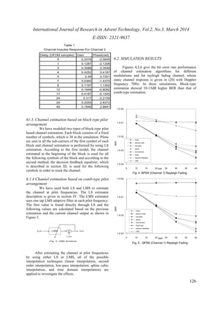
The comb-type channel estimation with low
1.E+00
1.E-01
1.E-02
pass interpolation achieves the best performance among
all the estimation techniques for BPSK, QPSK and
16QAM modulation. The performance among comb-type
channel estimation techniques usually ranges from
the best to the worst as follows: low-pass, spline, time-domain,
second-order and linear. The result was
expected since the low-pass interpolation used in
simulation does the interpolation such that the mean-square
error between the interpolated points and their
ideal values is minimized. These results are also
consistent with those obtained in [3] and [4].
7. CONCLUSION
In this paper, a full review of block-type and
comb-type pilot based channel estimation is given.
Channel estimation based on block-type pilot
arrangement with or without decision feedback
equalizer is described. Channel estimation based on
comb-type pilot arrangement is presented by giving the
channel estimation methods at the pilot frequencies and
the interpolation of the channel at data frequencies. The
simulation results show that comb-type pilot based
channel estimation with low-pass interpolation performs
the best among all channel estimation algorithms. This
was expected since the comb-type pilot arrangement
allows the tracking of fast fading channel and low-pass
interpolation does the interpolation such that the mean-square
error between the interpolated points and their
ideal values is minimized. In addition, for low Doppler
frequencies, the performance of decision feedback
estimation is observed to be slightly worse than that of
the best estimation. Therefore, some performance
degradation can be tolerated for higher data bit rate for
low Doppler spread channels although low-pass
interpolation comb-type channel estimation is more
robust for Doppler frequency increase.
REFERENCES
[1] J.-J van de Beek, O. Edfors, M. Sandell, S.K.
Wilson and P.O. Borjesson, “ On channel
estimation in OFDM systems” in Proc. IEEE 45th
Vehicular Technology Conference, Chicago, IL,
Jul. 1995, pp. 815-819
[2] O. Edfors, M. Sandell, J.-J van de Beek, S.K.
Wilson and P.O. Borjesson, “OFDM channel
estimation by singular value decomposition” in
Proc. IEEE 46th Vehicular Technology Conference,
Atlanta, GA, USA, Apr. 1996, pp. 923-927
[3] M. Hsieh and C. Wei, “Channel estimation for
OFDM systems based on comb-type pilot
arrangement in frequency selective fading
channels” in IEEE Transactions on Consumer
Electronics, vol. 44, no.1, February 1998
[4] R. Steele, Mobile Radio Communications, London,
England, Pentech Press Limited, 1992
[5] U. Reimers, “Digital video broadcasting,” IEEE
Communications Magazine, vol. 36, no. 6, pp. 104-
110, June 1998.
[6] L. J. Cimini, Jr., “Analysis and simulation of a
digital mobile channel using orthogonal frequency
division multiplexing,” IEEE Trans. Commun.,
vol.33, no. 7, pp. 665-675, July 1985.
[7] Y. Zhao and A. Huang, “A novel channel
estimation method for OFDM Mobile
Communications Systems based on pilot signals
and transform domain processing”, in Proc. IEEE
47th Vehicular Technology Conference, Phoenix,
USA, May 1997, pp. 2089-2093
[8] A. V. Oppenheim and R. W. Schafer, Discrete-
Time Signal Processing, New Jersey, Prentice-Hall
Inc., 1999
[9] Digital video broadcasting (DVB): Framing,
channel coding and modulation for digital
terrestrial television, Draft ETSI EN300 744
V1.3.1 (2000-08).
[10] Y. Li, “Pilot-Symbol-Aided Channel Estimation for
OFDM in Wireless Systems”, in IEEE Transactions
on Vehicular Technology, vol. 49, no.4, July 2000.
1.E-03
5 10 15 20 25 30 35 40
BER
SNR
Fig. 6. 16QAM (Channel 1) Rayleigh Fading