Integer , Goal and Non linear Programming Model

1. Chapter 6
Integer, Goal, and Nonlinear
Programming Models
© 2007 Pearson Education

2. Variations of Basic
Linear Programming
• Integer Programming
• Goal Programming
• Nonlinear Programming

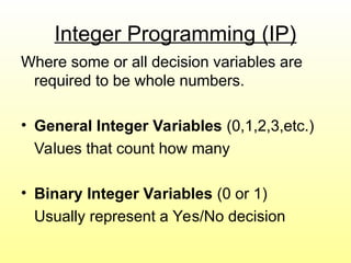
3. Integer Programming (IP)
Where some or all decision variables are
required to be whole numbers.
• General Integer Variables (0,1,2,3,etc.)
Values that count how many
• Binary Integer Variables (0 or 1)
Usually represent a Yes/No decision

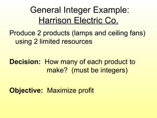
4. General Integer Example:
Harrison Electric Co.
Produce 2 products (lamps and ceiling fans)
using 2 limited resources
Decision: How many of each product to
make? (must be integers)
Objective: Maximize profit

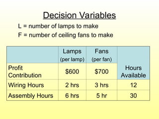
5. Decision Variables
L = number of lamps to make
F = number of ceiling fans to make
Lamps
(per lamp)
Fans
(per fan)
Hours
Available
Profit
Contribution
$600 $700
Wiring Hours 2 hrs 3 hrs 12
Assembly Hours 6 hrs 5 hr 30

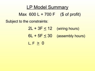
6. LP Model Summary
Max 600 L + 700 F ($ of profit)
Subject to the constraints:
2L + 3F < 12 (wiring hours)
6L + 5F < 30 (assembly hours)
L, F > 0

7. Graphical Solution

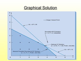
8. Properties of Integer Solutions
• Rounding off the LP solution might not
yield the optimal IP solution
• The IP objective function value is usually
worse than the LP value
• IP solutions are usually not at corner
points

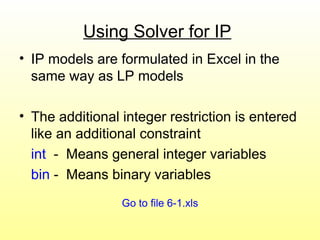
9. Using Solver for IP
• IP models are formulated in Excel in the
same way as LP models
• The additional integer restriction is entered
like an additional constraint
int - Means general integer variables
bin - Means binary variables
Go to file 6-1.xls

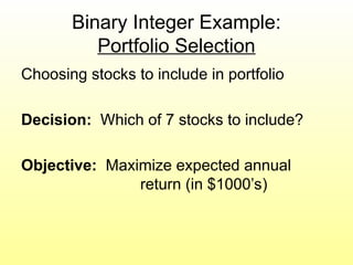
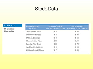
10. Binary Integer Example:
Portfolio Selection
Choosing stocks to include in portfolio
Decision: Which of 7 stocks to include?
Objective: Maximize expected annual
return (in $1000’s)

11. Stock Data

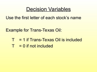
12. Decision Variables
Use the first letter of each stock’s name
Example for Trans-Texas Oil:
T = 1 if Trans-Texas Oil is included
T = 0 if not included

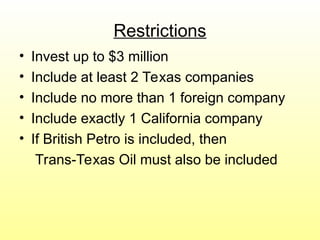
13. Restrictions
• Invest up to $3 million
• Include at least 2 Texas companies
• Include no more than 1 foreign company
• Include exactly 1 California company
• If British Petro is included, then
Trans-Texas Oil must also be included

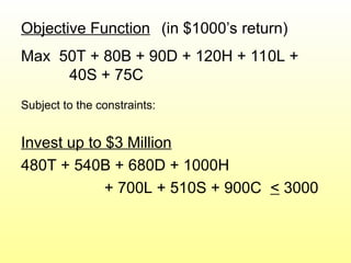
14. Objective Function (in $1000’s return)
Max 50T + 80B + 90D + 120H + 110L +
40S + 75C
Subject to the constraints:
Invest up to $3 Million
480T + 540B + 680D + 1000H
+ 700L + 510S + 900C < 3000

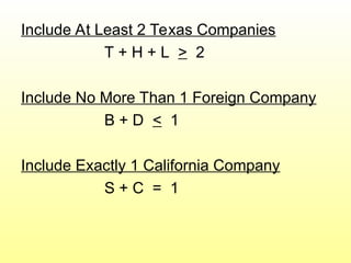
15. Include At Least 2 Texas Companies
T + H + L > 2
Include No More Than 1 Foreign Company
B + D < 1
Include Exactly 1 California Company
S + C = 1

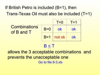
16. If British Petro is included (B=1), then
Trans-Texas Oil must also be included (T=1)
T=0 T=1
B=0 ok ok
B=1 not ok ok
B < T
allows the 3 acceptable combinations and
prevents the unacceptable one
Go to file 6-3.xls
Combinations
of B and T

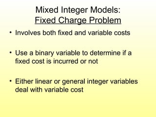
17. Mixed Integer Models:
Fixed Charge Problem
• Involves both fixed and variable costs
• Use a binary variable to determine if a
fixed cost is incurred or not
• Either linear or general integer variables
deal with variable cost

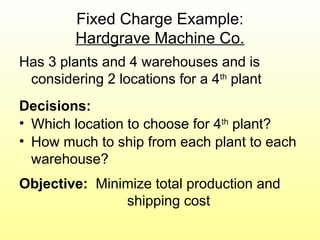
18. Fixed Charge Example:
Hardgrave Machine Co.
Has 3 plants and 4 warehouses and is
considering 2 locations for a 4th
plant
Decisions:
• Which location to choose for 4th
plant?
• How much to ship from each plant to each
warehouse?
Objective: Minimize total production and
shipping cost

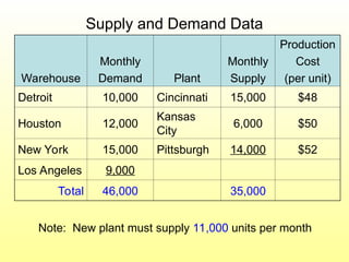
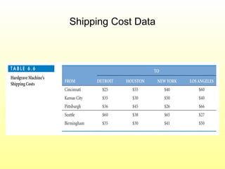
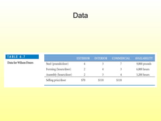
19. Supply and Demand Data
Warehouse
Monthly
Demand Plant
Monthly
Supply
Production
Cost
(per unit)
Detroit 10,000 Cincinnati 15,000 $48
Houston 12,000
Kansas
City
6,000 $50
New York 15,000 Pittsburgh 14,000 $52
Los Angeles 9,000
Total 46,000 35,000
Note: New plant must supply 11,000 units per month

20. Production Cost
(per unit)
Fixed Cost
(per month)
Seattle $53 $400,000
Birmingham $49 $325,000
Possible Locations for New Plant

21. Shipping Cost Data

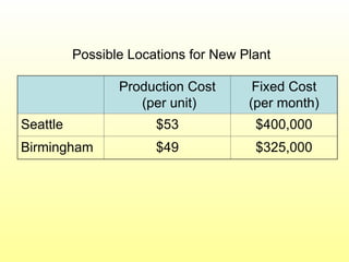
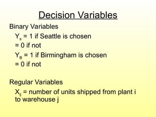
22. Decision Variables
Binary Variables
Ys = 1 if Seattle is chosen
= 0 if not
YB = 1 if Birmingham is chosen
= 0 if not
Regular Variables
Xij = number of units shipped from plant i
to warehouse j

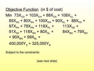
23. Objective Function (in $ of cost)
Min 73XCD + 103XCH + 88XCN + 108XCL +
85XKD + 80XKH + 100XKN + 90XKL + 88XPD +
97XPH + 78XPN + 118XPL + 113XSD +
91XSH + 118XSN + 80XSL + 84XBD + 79XBH
+ 90XBN + 99XBL +
400,000YS + 325,000YB
Subject to the constraints:
(see next slide)

24. Supply Constraints
-(XCD + XCH + XCN + XCL) = -15,000 (Cincinnati)
-(XKD + XKH + XKN + XKL) = - 6,000 (Kansas City)
-(XPD + XPH + XPN + XPL) = -15,000 (Pittsburgh)
Possible Locations for New Plant
-(XSD + XSH + XSN + XSL) = -11,000YS (Seattle)
-(XBD + XBH + XBN + XBL) = -11,000YB (B’ham)

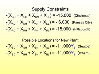
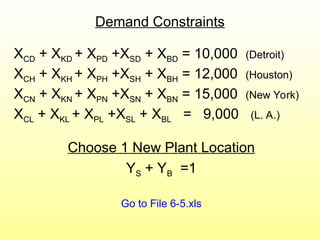
25. Demand Constraints
XCD + XKD + XPD +XSD + XBD = 10,000 (Detroit)
XCH + XKH + XPH +XSH + XBH = 12,000 (Houston)
XCN + XKN + XPN +XSN + XBN = 15,000 (New York)
XCL + XKL + XPL +XSL + XBL = 9,000 (L. A.)
Choose 1 New Plant Location
YS + YB =1
Go to File 6-5.xls

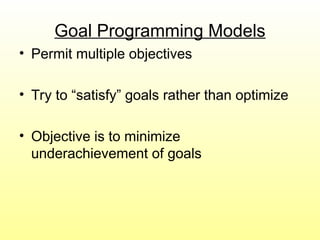
26. Goal Programming Models
• Permit multiple objectives
• Try to “satisfy” goals rather than optimize
• Objective is to minimize
underachievement of goals

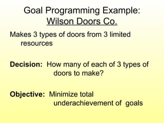
27. Goal Programming Example:
Wilson Doors Co.
Makes 3 types of doors from 3 limited
resources
Decision: How many of each of 3 types of
doors to make?
Objective: Minimize total
underachievement of goals

28. Data

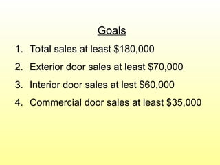
29. Goals
1. Total sales at least $180,000
2. Exterior door sales at least $70,000
3. Interior door sales at lest $60,000
4. Commercial door sales at least $35,000

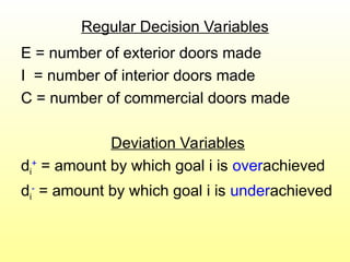
30. Regular Decision Variables
E = number of exterior doors made
I = number of interior doors made
C = number of commercial doors made
Deviation Variables
di
+
= amount by which goal i is overachieved
di
-
= amount by which goal i is underachieved

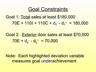
31. Goal Constraints
Goal 1: Total sales at least $180,000
70E + 110I + 110C + dT
-
- dT
+
= 180,000
Goal 2: Exterior door sales at least $70,000
70E + dE
-
- dE
+
= 70,000
Note: Each highlighted deviation variable
measures goal underachievement

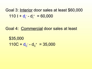
32. Goal 3: Interior door sales at least $60,000
110 I + dI
-
- dI
+
= 60,000
Goal 4: Commercial door sales at least
$35,000
110C + dC
-
- dC
+
= 35,000

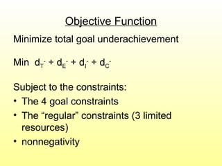
33. Objective Function
Minimize total goal underachievement
Min dT
-
+ dE
-
+ dI
-
+ dC
-
Subject to the constraints:
• The 4 goal constraints
• The “regular” constraints (3 limited
resources)
• nonnegativity

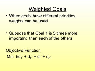
34. Weighted Goals
• When goals have different priorities,
weights can be used
• Suppose that Goal 1 is 5 times more
important than each of the others
Objective Function
Min 5dT
-
+ dE
-
+ dI
-
+ dC
-

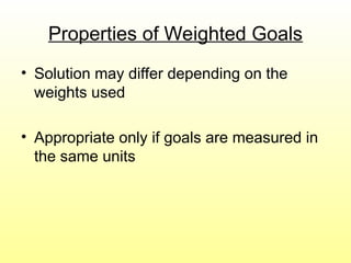
35. Properties of Weighted Goals
• Solution may differ depending on the
weights used
• Appropriate only if goals are measured in
the same units

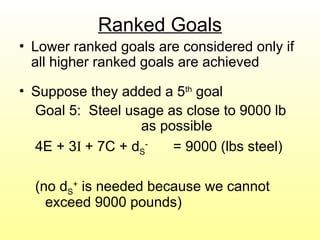
36. Ranked Goals
• Lower ranked goals are considered only if
all higher ranked goals are achieved
• Suppose they added a 5th
goal
Goal 5: Steel usage as close to 9000 lb
as possible
4E + 3I + 7C + dS
-
= 9000 (lbs steel)
(no dS
+
is needed because we cannot
exceed 9000 pounds)

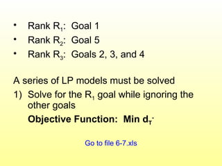
37. • Rank R1: Goal 1
• Rank R2: Goal 5
• Rank R3: Goals 2, 3, and 4
A series of LP models must be solved
1) Solve for the R1 goal while ignoring the
other goals
Objective Function: Min dT
-
Go to file 6-7.xls

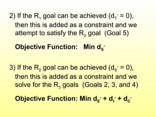
38. 2) If the R1 goal can be achieved (dT
-
= 0),
then this is added as a constraint and we
attempt to satisfy the R2 goal (Goal 5)
Objective Function: Min dS
-
3) If the R2 goal can be achieved (dS
-
= 0),
then this is added as a constraint and we
solve for the R3 goals (Goals 2, 3, and 4)
Objective Function: Min dE
-
+ dI
-
+ dC
-

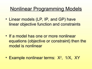
39. Nonlinear Programming Models
• Linear models (LP, IP, and GP) have
linear objective function and constraints
• If a model has one or more nonlinear
equations (objective or constraint) then the
model is nonlinear
• Example nonlinear terms: X2
, 1/X, XY

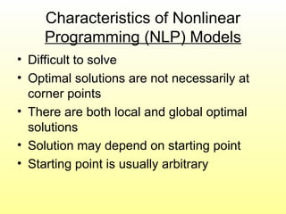
40. Characteristics of Nonlinear
Programming (NLP) Models
• Difficult to solve
• Optimal solutions are not necessarily at
corner points
• There are both local and global optimal
solutions
• Solution may depend on starting point
• Starting point is usually arbitrary

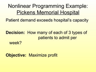
41. Nonlinear Programming Example:
Pickens Memorial Hospital
Patient demand exceeds hospital’s capacity
Decision: How many of each of 3 types of
patients to admit per
week?
Objective: Maximize profit

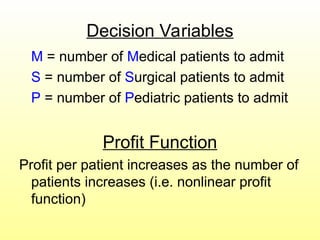
42. Decision Variables
M = number of Medical patients to admit
S = number of Surgical patients to admit
P = number of Pediatric patients to admit
Profit Function
Profit per patient increases as the number of
patients increases (i.e. nonlinear profit
function)

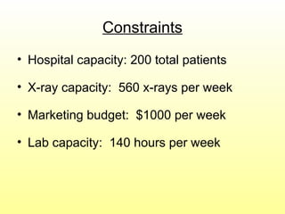
43. Constraints
• Hospital capacity: 200 total patients
• X-ray capacity: 560 x-rays per week
• Marketing budget: $1000 per week
• Lab capacity: 140 hours per week

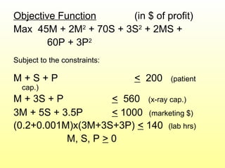
44. Objective Function (in $ of profit)
Max 45M + 2M2
+ 70S + 3S2
+ 2MS +
60P + 3P2
Subject to the constraints:
M + S + P < 200 (patient
cap.)
M + 3S + P < 560 (x-ray cap.)
3M + 5S + 3.5P < 1000 (marketing $)
(0.2+0.001M)x(3M+3S+3P) < 140 (lab hrs)
M, S, P > 0

45. Using Solver for NLP Models
• Solver uses the Generalized Reduced
Gradient (GRG) method
• GRG uses the path of steepest ascent (or
descent)
• Moves from one feasible solution to
another until the objective function value
stops improving (converges)
Go to file 6-8.xls