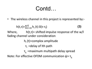
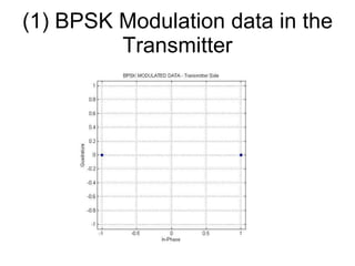
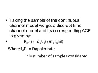
![Transmitter Section First the high serial data rate input with sampling time T s is modulated using any digital modulation technique (BPSK, QAM, QPSK etc), to give digital symbols b m [k]. Next the modulated serial data is converted to low rate parallel data streams (M) using S/P converter. Due to this parallel conversion, the effective symbol duration is increased to T= MT s Where index k=I,2,….. is the symbol interval and m=0,1,….M-1 are the number of sub-channels.](https://image.slidesharecdn.com/finalppt-111212005827-phpapp01/85/Final-ppt-7-320.jpg)
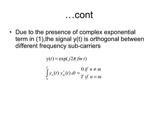
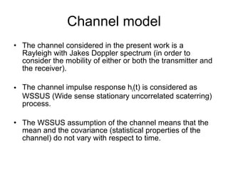
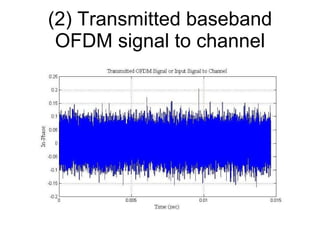
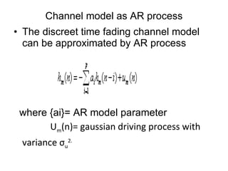
![… cont. Referring to Fig-3 the symbols b m [k] are modulated onto different sub-carriers using IFFT block, which is mathematically expressed as y(t)=∑ M-1 m=0 b m [k]exp(j2 π mt/T), for kT ≤ t ≤ (k+1)T -----(1) y(t) indicates modulated multiplexed signal that will be transmitted by OFDM transmitter.](https://image.slidesharecdn.com/finalppt-111212005827-phpapp01/85/Final-ppt-8-320.jpg)
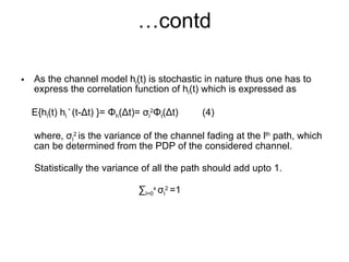
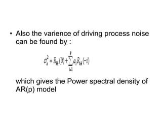
![… To mitigate the effect of ISI, signal y(t) in (1) is added with a cyclic prefix thus the mathematical expression of y(t) becomes y(t)=∑ M-1 m=0 b m [k]exp(j2 π mt/T), for - Ψ +kT ≤ t ≤ (k+1)T --------------(2) where Ψ is guard interval.](https://image.slidesharecdn.com/finalppt-111212005827-phpapp01/85/Final-ppt-10-320.jpg)
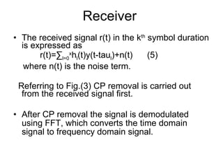
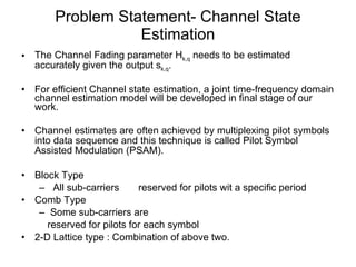
![Determination of AR parameter The AR parameter are obtained by Yule-Walker equation: R hh θ= -r h Where R hh = fading channel ACF matrix of pxp θ = [ a 1, a 2 , ….a p ] T = px1 vector storing the AR parameter r h = px1 channel ACF vector](https://image.slidesharecdn.com/finalppt-111212005827-phpapp01/85/Final-ppt-31-320.jpg)

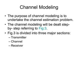
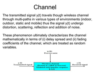
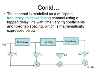
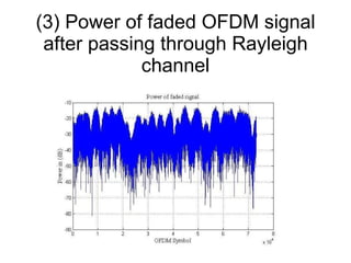
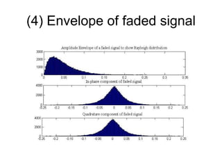
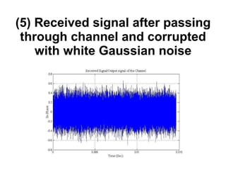
The document discusses channel modeling and Kalman filter-based estimation for OFDM wireless communication systems. It provides an introduction to OFDM systems and outlines the channel modeling process, including modeling the channel as a multipath frequency selective fading channel using a tapped delay line. It also discusses implementing channel estimation using a Kalman filter and presenting results on simulating OFDM signal transmission through a Rayleigh fading channel. The goal is to accurately estimate the channel fading parameters using a joint time-frequency domain estimation model.