Downloaded 20 times


![Principles of Communication Prof. V. Venkata Rao
Indian Institute of Technology Madras
6.8
s
s
f
W f W
2
≤ ≤ − . Then, ( )h t the impulse response of the ideal lowpass filter
is, ( ) ( )sh t T W c W t' '2 sin 2= . As ( ) ( ) ( )sx t x t h t= ∗ and sW T'
2 1= , we have
( ) ( ) ( )s s
n
x t x nT c W t nT'sin 2
∞
= − ∞
⎡ ⎤= −
⎢ ⎥⎣ ⎦
∑ (6.3a)
If the sampling is done at the Nyquist rate, then W W' = and Eq. 6.3(a) reduces
to
( ) ( )
n
n
x t x c W t n
W
sin 2
2
∞
= − ∞
⎛ ⎞
= −⎜ ⎟
⎝ ⎠
∑ (6.3b)
That is, the impulse response of the ideal lowpass filter, which is a ( )csin
function, acts as the interpolating function and given the input,
( ) ( ){ }s sx nT t nTδ − , it interpolates the samples and produces ( )x t for all t .
Note that ( )sx t represents a sequence of impulses. The weight of the
impulse at st nT= is equal to ( )sx nT . In order that the sampler output be equal
to ( )sx nT , we require conceptually, the impulse modulator to be followed by a
unit that converts impulses into a sequence of sample values which are basically
a sequence of numbers. In [1], such a scheme has been termed as an “ideal C-
to-D converter”. For simplicity, we assume that the output of the sampler
represents the sample sequence ( ){ }sx nT .
To reconstruct ( )x t from ( ){ }sx nT , we have to perform the inverse
operation, namely, convert the sample sequence to an impulse train. This has
been termed as an “ideal D-to-C converter in [1]. We will assume that the
reconstruction filter in Fig. 6.1 will take care of this aspect, if necessary.](https://image.slidesharecdn.com/basebandtransmission-180528223405/85/Baseband-transmission-8-320.jpg)


![Principles of Communication Prof. V. Venkata Rao
Indian Institute of Technology Madras
6.43
variety. When x I6∈ , ( )C x I6
'∈ and the input to the UQ will be in the range
( ), 2∆ ∆ . Then the quantizer output is
3
2
∆
. When kx I∈ , the compressor
characteristic ( )C x , may be approximated by a straight line segment with a
slope equal to
k
x
L
max2
∆
, where k∆ is the width of the interval kI . That is,
( )
( )
k
k
dC x x
C x x I
d x L
max2' ,= ∈
∆
As ( )C x' is maximum at the origin, the equivalent step size is smallest at
x 0= and k∆ is the largest at x xmax= . If L is large, the input PDF ( )Xf x can
be treated to be approximately constant in any interval kI k L, 1, ,= ⋅⋅⋅ . Note
that we are assuming that the input is bounded in practice to a value xmax , even
if the PDF should have a long tail. We also assume that ( )Xf x is symmetric; that
is ( ) ( )X Xf x f x= − . Let ( ) ( )X X kf x f yconstant = , kx I∈ , where
k k
k
x x
y
1
2
+ +
=
and k k k klength of I x x1+∆ = = −
Then, [ ] ( )
k
k
x
k k X
x
P P x I f x d x
1+
= ∈ = ∫ , and,
L
k
k
P
1
1
=
=∑
Let kq denote the quantization error when kx I∈ .
That is, ( )k kq QZ x x x I,= − ∈
k ky x x I,= − ∈](https://image.slidesharecdn.com/basebandtransmission-180528223405/85/Baseband-transmission-43-320.jpg)


![Principles of Communication Prof. V. Venkata Rao
Indian Institute of Technology Madras
6.55
Exercise 6.7
Let the input to µ-law compander be the sample function ( )jx t of a random
process ( ) ( )mX t f tcos 2= π + Θ where Θ is uniformly distributed in the
range ( )0, 2π . Find the ( ) q
SNR 0,
expected of the scheme.
Note that samples of ( )jx t will have the PDF,
( )X
x
f x x
otherwise
2
1
, 1
1
0 ,
⎧
≤⎪
= π −⎨
⎪
⎩
Answer: ( )
( )q
L
SNR
12 2
0,
3
1
2 ln 1 2
−
⎡ ⎤⎛ ⎞µ µ 4µ
= + +⎜ ⎟ ⎢ ⎥⎜ ⎟+ µ π⎢ ⎥⎝ ⎠ ⎣ ⎦
Note that if
2
1
2
µ
>> µ >> , we have ( )
( )
q
L
SNR
2
20,
3
ln 1⎡ ⎤+ µ⎣ ⎦
Exercise 6.8
Show that for values of x such that A x xmax>> , ( ) q
SNR 0,
of the
A-law PCM is given by
( ) q
SNR R0,
6= + α
where [ ]A104.77 20 log 1 lnα = − +
Exercise 6.9
Let ( )C x denote the compression characteristic. Then
( )
x
dC x
d x 0→
is called the companding gain, cG . Show that
a) cG (A-law) with A 87.56= is 15.71 (and hence cG1020 log 24 dB)
b) cG (µ-law) with 255µ = is 46.02 (and hence cG1020 log 33 dB.)](https://image.slidesharecdn.com/basebandtransmission-180528223405/85/Baseband-transmission-55-320.jpg)


![Principles of Communication Prof. V. Venkata Rao
Indian Institute of Technology Madras
6.63
Let ( )p t be rectangular pulse of unit amplitude and duration bT sec. Then, ( )P f
is ( ) ( )b bP f T c f Tsin=
and ( )XS f can be written as
( ) ( ) ( ) [ ]b b
X b b b
n
a T a T
S f c f T c f T j nf T
2 2
2 2
sin sin exp 2
4 4
∞
= − ∞
⎛ ⎞
= + π⎜ ⎟⎜ ⎟
⎝ ⎠
∑
But from Poisson's formula,
[ ]b
b bn m
m
j nf T f
T T
1
exp 2
∞ ∞
= − ∞ = − ∞
⎛ ⎞
π = δ −⎜ ⎟
⎝ ⎠
∑ ∑
Noting that ( )bc f Tsin has nulls at ( )X
b
n
f n S f
T
, 1, 2, ,= = ± ± ⋅⋅⋅ can be
simplified to
( ) ( ) ( )b
X b
a T a
S f c f T f
2 2
2
sin
4 4
= + δ (6.23a)
If the duration of ( )p t is less than bT , then we have unipolar RZ sequence. If
( )p t is of duration bT
2
seconds, then ( )XS f reduces to
( ) b b
X
b bm
a T f T m
S f c f
T T
2
2 1
sin 1
16 2
∞
= − ∞
⎡ ⎤⎛ ⎞⎛ ⎞
= + δ −⎢ ⎥⎜ ⎟⎜ ⎟
⎝ ⎠ ⎢ ⎥⎝ ⎠⎣ ⎦
∑ (6.23b)
From equation 6.23(b) it follows that unipolar RZ signaling has discrete spectral
components at
b b
f
T T
1 3
0, ,= ± etc. A plot of Eq. 6.23(b) is shown in Fig. 6.34(a).
6.7.2 Polar Format
Assuming, [ ] [ ]k kP A a P A a
1
2
= + = = − = and 0's and 1's of the binary
data sequence are statistically independent; it is easy to show,
( )A
a n
R n
n
2
, 0
0 , 0
⎧ =⎪
= ⎨
≠⎪⎩](https://image.slidesharecdn.com/basebandtransmission-180528223405/85/Baseband-transmission-63-320.jpg)
![Principles of Communication Prof. V. Venkata Rao
Indian Institute of Technology Madras
6.64
With ( )p t being a rectangular pulse of duration bT sec. (NRZ case), we have
( ) ( )X b bS f a T c f T2 2
sin= (6.24a)
The PSD for the case when ( )p t is duration of bT
2
(RZ case), is given by
( ) b b
X
T f T
S f a c2 2
sin
4 2
⎛ ⎞
= ⎜ ⎟
⎝ ⎠
(6.24b)
6.7.3 Bipolar Format
Bipolar format has three levels: a, 0 and ( )a− . Assuming that 1's and 0's
are equally likely, we have [ ] [ ]k kP A a P A a
1
4
= = = − = and
[ ]kP A
1
0
2
= = . We shall now compute the autocorrelation function of a bipolar
sequence.
( ) ( ) ( ) ( ) ( )AR a a a a
1 1 1
0 0 0
4 4 2
= ⋅ + − − + ⋅
a2
2
=
To compute ( )AR 1 , we have to consider the four two bit sequences, namely, 00,
01, 10, 11. As the binary ‘0’ is represented by zero volts, we have only one non-
zero product, corresponding to the binary sequence (11). As each one of these
two bit sequences occur with a probability
1
4
, we have
( )A
a
R
2
1
4
= −
To compute ( )AR n , for n 2≥ , again we have to take into account only those
binary n-tuples which have ‘1’ in the first and last position, which will result in the
product a2
± . It is not difficult to see that, in these product terms, there are as
many terms with a2
− as there are with a2
which implies that the sum of the
product terms would be zero. (For example, if we take the binary 3-tuples, only](https://image.slidesharecdn.com/basebandtransmission-180528223405/85/Baseband-transmission-64-320.jpg)


![Principles of Communication Prof. V. Venkata Rao
Indian Institute of Technology Madras
6.74
( ) ( ) ( )
M
i
i
E n E X n X n i
2
2
1=
⎧ ⎫⎡ ⎤⎪ ⎪⎡ ⎤ = − α −⎢ ⎥⎨ ⎬⎣ ⎦ ⎢ ⎥⎪ ⎪⎣ ⎦⎩ ⎭
∑E is minimized. To obtain the
optimum ( )M1 2, , ,= α α ⋅⋅⋅ αα , let us introduce some notation. Let
n i n jE X X− −⎡ ⎤
⎣ ⎦ be denoted by ( )xr j i− and let
( ) ( ) ( )
( ) ( ) ( )
( ) ( ) ( )
x x x
x x x
X
x x x
r r r M
r r r M
R
r M r M r
0 1 1
1 0 2
1 2 0
⎡ ⎤⋅⋅⋅ −
⎢ ⎥
⋅⋅⋅ −⎢ ⎥
⎢ ⎥⋅
= ⎢ ⎥
⋅⎢ ⎥
⎢ ⎥⋅
⎢ ⎥
− − ⋅⋅⋅⎢ ⎥⎣ ⎦
( )
( )
( )
x
x
X
x
r
r
r M
1
2
⎡ ⎤
⎢ ⎥
⎢ ⎥
⎢ ⎥⋅
= ⎢ ⎥
⋅⎢ ⎥
⎢ ⎥⋅
⎢ ⎥
⎢ ⎥⎣ ⎦
t
Then, it has been shown that (see Haykin [2], Jayant and Noll [3]), the optimum
predictor vector
( ) ( )T T
Mopt 1 2, , ,= α α ⋅⋅⋅ αα , where the superscript T denotes the
transpose, is given by
( )T
XXopt
R 1−
=α t (6.33)
and ( ) ( ) ( )
M
X i X
i
r r i2
min
1
0ε
=
σ = − α∑ (6.34a)
M
X i i
i
2
1
1
=
⎡ ⎤
= σ − α ρ⎢ ⎥
⎢ ⎥⎣ ⎦
∑ (6.34b)
where
( )
( )
X
j
X
r j
r 0
ρ = (6.34c)](https://image.slidesharecdn.com/basebandtransmission-180528223405/85/Baseband-transmission-74-320.jpg)


![Principles of Communication Prof. V. Venkata Rao
Indian Institute of Technology Madras
6.78
sequence ( )e n , indicated by ( )p
SNR . A value of pG greater than unity
represents the gain in SNR that is due to the prediction operation of the DPCM
scheme.
x X
p
M
X i i
i
G
2 2
2
2
1
1
ε
=
σ σ
= =
⎡ ⎤σ
σ − α ρ⎢ ⎥
⎢ ⎥⎣ ⎦
∑
M
i i
i 1
1
1
=
=
− α ρ∑
(6.39b)
where iα ’s are the optimum predictor coefficients. Jayant and Noll [3], after a
great deal of empirical studies, have reported that for voice signals pG can be of
the order of 5-10 dB. In the case of TV video signals, which have much higher
correlation than voice, it is possible to achieve a prediction gain of about 12 dB.
With a 12 dB prediction gain, it is possible to reduce the number of bits/ sample
by 2.
Example 6.16
The designer of a DPCM system finds by experimental means that a third
order predictor gives the required prediction gain. Let piα denote the th
i
coefficient of an optimum th
p order predictor. Given that 11
2
3
α = − , 22
1
5
α =
and 33
1
4
α = , find the prediction gain given by the third order predictor. you can
assume ( )xr 0 1= .
We have
( )
( )
x
x
r
r
11 1
1 2
0 3
α = = ρ = −
2
2 1
22 2
11
ρ − ρ
α =
− ρ
(See Eq. 6.35(b))](https://image.slidesharecdn.com/basebandtransmission-180528223405/85/Baseband-transmission-78-320.jpg)

![Principles of Communication Prof. V. Venkata Rao
Indian Institute of Technology Madras
6.80
inputs. Evidently, we can expect better performance from a ADPCM than a
scheme that is fixed. 32 kbps (8 kHz sampling, 4 bits/sample coding) ADPCM
coders for speech have been developed whose performance is quite comparable
with that of 64 kbps companded PCM. Also 64 kbps DPCM has been developed
for encoding audio signals with a bandwidth of 7 kHz. This coder uses a
sampling rate of 16 kHz and a quantizer with 16 levels. Details can be found in
Benevuto et al [4] and Decina and Modena [5].
At the start of the section, we had mentioned that DPCM is a special case
of PCM. If we want, we could treat PCM to be a special case of DPCM where the
predictor output is always zero!
6.9 Delta Modulation
Delta modulation, like DPCM is a predictive waveform coding technique
and can be considered as a special case of DPCM. It uses the simplest possible
quantizer, namely a two level (one bit) quantizer. The price paid for achieving the
simplicity of the quantizer is the increased sampling rate (much higher than the
Nyquist rate) and the possibility of slope-overload distortion in the waveform
reconstruction, as explained in greater detail later on in this section.
In DM, the analog signal is highly over-sampled in order to increase the
adjacent sample correlation. The implication of this is that there is very little
change in two adjacent samples, thereby enabling us to use a simple one bit
quantizer, which like in DPCM, acts on the difference (prediction error) signals.
In its original form, the DM coder approximates an input time function by a
series of linear segments of constant slope. Such a coder is therefore referred to
as a Linear (or non-adaptive) Delta Modulator (LDM). Subsequent developments
have resulted in delta modulators where the slope of the approximating function](https://image.slidesharecdn.com/basebandtransmission-180528223405/85/Baseband-transmission-80-320.jpg)


![Principles of Communication Prof. V. Venkata Rao
Indian Institute of Technology Madras
6.92
[ ] [ ]
1 1
1953125 50781250
750 1500
= +
7812.5 33854.16 41666.66= + =
rmsB 204.12=
opt
2 3 204.12
7500
π × ×
δ =
0.512=
6.9.2 Adaptive delta modulation
Consider Fig. 6.40. We see that for a given value of F , there is an
optimum value of ξ which gives rise to maximum ( ) q
SNR 0,
from a DM coder.
Let us now change ξ from optξ by varying Xσ with δ fixed. We then find that
the range of Xσ for which near about this maximum ( ) q
SNR 0,
is possible is very
limited. (This situation is analogous to the uncompanded PCM). Adaptive Delta
Modulation, a modification of LDM, is a scheme that circumvents this deficiency
of LDM.
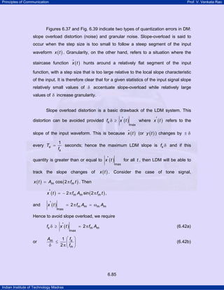
The principle of ADM is illustrated in Fig. 6.41. Here the step size ∆ of the
quantizer is not a constant but varies with time. We shall denote by
( ) ( )n n2∆ = δ , the step size at ( )st nT n= ⋅ δ increases during a steep
segment of the input and decreases when the modulator is quantizing a slowly
varying segment of x(t). A specific step-size adaptation scheme is discussed in
detail later on in this section.
The adaptive step size control which forms the basis of an ADM scheme
can be classified in various ways such as: discrete or continuous; instantaneous
or syllabic (fairly gradual change); forward or backward. Here, we shall describe
an adaptation scheme that is backward, instantaneous and discrete. For
extensive coverage on ADM, the reader is referred to Jayant and Noll [3].](https://image.slidesharecdn.com/basebandtransmission-180528223405/85/Baseband-transmission-92-320.jpg)


![Principles of Communication Prof. V. Venkata Rao
Indian Institute of Technology Madras
6.96
Instantaneously adapting delta modulators (such as the scheme described
above) are more vulnerable to channel noise than the slowly adapting or linear
coders. Therefore, although instantaneously adapting delta modulators are very
simple and efficient (SNR-wise) in a relatively noise-free environments (say, bit
error probability 4
10−
< ), a number of syllabically adaptive delta modulators
have been designed for use over noisy channels and these coders are
particularly attractive for low-bit-rate ( 20< k bits/sec) applications. For details on
syllabic adaptation, the reader is referred to [3].](https://image.slidesharecdn.com/basebandtransmission-180528223405/85/Baseband-transmission-96-320.jpg)
![Principles of Communication Prof. V. Venkata Rao
Indian Institute of Technology Madras
6.97
Appendix A6.1
PSD of a waveform process with discrete amplitudes
A sequence of symbols are transmitted using some basic pulse ( )p t . Let
the resulting waveform process be denoted by ( )X t , given by
( ) ( )k d
k
X t A p t kT T
∞
= − ∞
= − −∑ (A6.1)
kA ’s are discrete random variables, and dT 1
is a random variable uniformly
distributed in the interval
T T
,
2 2
⎛ ⎞
−⎜ ⎟
⎝ ⎠
. kA ’s are independent of dT . T is the
symbol duration. (For the case of binary transmission, we use bT instead of T ;
bit rate
bT
1
= .) We shall assume that the autocorrelation of the discrete
amplitude sequence is a function of only the time difference. That is,
( )k k n A k k nE A A R n E A A+ −⎡ ⎤ ⎡ ⎤= =⎣ ⎦ ⎣ ⎦ (A6.2)
With these assumptions, we shall derive an expression for the
autocorrelation of the process ( )X t
( ) ( ) ( )XR t t E X t + X t, ⎡ ⎤+ τ = τ⎣ ⎦
( ) ( )k j d d
k j
E A A p t kT T p t jT T
∞ ∞
= − ∞ = − ∞
⎡ ⎤
= + τ − − − −⎢ ⎥
⎢ ⎥⎣ ⎦
∑ ∑
Let j k n= + for some n . Then,
( ) ( ) ( )+
−
⎡ ⎤
⎢ ⎥
+ τ = α β⎢ ⎥
⎢ ⎥
⎢ ⎥⎣ ⎦
∑∑ ∫
T
X k k dn
k n T
R t t A A p p d t
T
2
2
1
,
where ( )dt kT tα = + τ − − and ( )dt jT tβ = − − .
1
For an alternative derivative for the PSD, without the random delay d
T in ( )X t , see [6].](https://image.slidesharecdn.com/basebandtransmission-180528223405/85/Baseband-transmission-97-320.jpg)


1) The document discusses digital transmission of analog signals using techniques like Pulse Code Modulation (PCM), Differential Pulse Code Modulation (DPCM), and Delta Modulation (DM). 2) PCM involves sampling the analog signal, quantizing the sample amplitudes, and encoding the quantized values into binary codewords. 3) Nyquist sampling theorem states that if a signal is bandlimited to W Hz, it can be reconstructed perfectly from samples taken at a rate of at least 2W samples/second.