Stopping Problems
Mohamed Seif, PhD student

ECE Department
October 2017The University of Arizona
Outline
October 2017The University of Arizona
• Motivation
• Preliminaries on Hypothesis Testing
• Basic Classic of Stopping Problems
• Sequential Probability Ratio Test
• Proposed Solution
•Application
2
Motivation
October 2017The University of Arizona
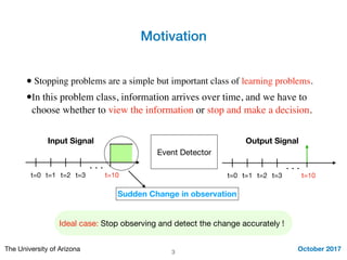
• Stopping problems are a simple but important class of learning problems.
•In this problem class, information arrives over time, and we have to
choose whether to view the information or stop and make a decision.
3
Event Detector
t=0 t=1 t=2 t=3
. . .
t=10
Input Signal
Sudden Change in observation
t=0 t=1 t=2 t=3
. . .
t=10
Ideal case: Stop observing and detect the change accurately !
Output Signal
Preliminaries on Hypothesis Testing
October 2017The University of Arizona
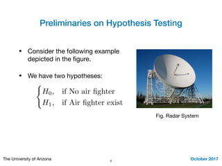
• Consider the following example
depicted in the figure.

• We have two hypotheses:
Fig. Radar System
(
H0, if No air fighter
H1, if Air fighter exist
4
Preliminaries on Hypothesis Testing (Cont’d)
October 2017The University of Arizona
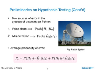
• Two sources of error in the
process of detecting air fighter:

1. False alarm 

2. Mis detection
Fig. Radar System
=) Prob{ ˆH1|H0}
=) Prob{ ˆH0|H1}
Pe = P(H0)P( ˆH1|H0) + P(H1)P( ˆH0|H1)
• Average probability of error:
5
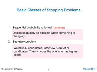
Basic Classes of Stopping Problems
October 2017The University of Arizona
1. Sequential probability ratio test (Talk focus) 

2. Secretary problem
6
We have N candidates, interview K out of N
candidates. Then, choose the one who has highest
score.
Decide as quickly as possible when something is
changing.
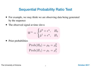
Wn
=
(
¯µ0
+ ✏n
, H0
¯µ1
+ ✏n
, H1
Sequential Probability Ratio Test
October 2017The University of Arizona 7
• For example, we may think we are observing data being generated
by the sequence
• The observed signal at time slot n
• Prior probabilities
Prob(H0) = ⇢0 = ⇢0
0
Prob(H1) = ⇢1 = ⇢0
1
Sequential Probability Ratio Test
October 2017The University of Arizona 8
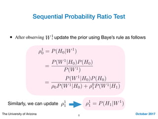
• After observing W1, update the prior using Baye’s rule as follows
⇢1
0 = P(H0|W1
)
=
P(W1
|H0)P(H0)
P(W1)
=
P(W1
|H0)P(H0)
⇢0P(W1|H0) + ⇢0
1P(W1|H1)
Similarly, we can update ⇢1
1 ⇢1
1 = P(H1|W1
)
Example
October 2017The University of Arizona
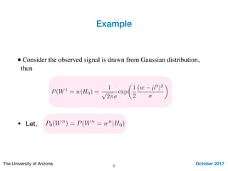
• Consider the observed signal is drawn from Gaussian distribution,
then
9
P(W1
= w|H0) =
1
p
2⇡
exp
✓
1
2
(w ¯µ0
)2
◆
• Let, P0(Wn
) = P(Wn
= wn
|H0)
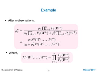
Example
October 2017The University of Arizona 10
⇢n
0 =
⇢0
Qn
k=1 P0(Wk
)
⇢0
Qn
k=1 P0(Wk) + ⇢0
1
Qn
k=1 P1(Wk)
• After n observations,
=
⇢0
n
(W1
, . . . , Wn
⇢0 + ⇢0
1
n(W1, . . . , Wn)
n
(W1
, . . . , Wn
) =
nY
k=1
P0(Wk
)
P1(Wk)
• Where,
)
Solution of the problem
October 2017The University of Arizona 11
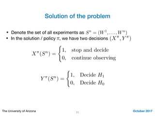
• Denote the set of all experiments as Sn
= (W1
, . . . , Wn
)
• In the solution / policy , we have two decisions (X⇡
, Y ⇡
)⇡
X⇡
(Sn
) =
(
1, stop and decide
0, continue observing
Y ⇡
(Sn
) =
(
1, Decide H1
0, Decide H0
Solution of the problem (Cont’d)
October 2017The University of Arizona 12
• Two sources of error can happen:
1. False alarm: stop and conclude H1
but the true is the null hypothesis H0
2. Mis detection: we did not pick up 

any change, i.e., concludeH0 but
H1the alternative hypothesis is true
P⇡
F = E [Y ⇡
(Sn
|H0)]
P⇡
M = E [1 Y ⇡
(Sn
|H1)]
Pe = (1 ⇢0)P⇡
F + ⇢0P⇡
M
• Average probability of error:
Solution of the problem (Cont’d)
October 2017The University of Arizona 13
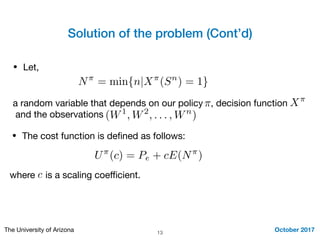
• Let,
N⇡
= min{n|X⇡
(Sn
) = 1}
a random variable that depends on our policy , decision function

and the observations
⇡ X⇡
(W1
, W2
, . . . , Wn
)
• The cost function is defined as follows:
U⇡
(c) = Pe + cE(N⇡
)
where is a scaling coefficient.c
Solution of the problem (Cont’d)
October 2017The University of Arizona 14
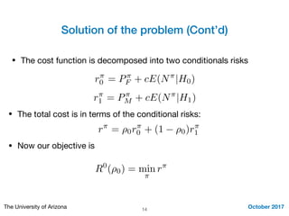
• The cost function is decomposed into two conditionals risks
r⇡
0 = P⇡
F + cE(N⇡
|H0)
r⇡
1 = P⇡
M + cE(N⇡
|H1)
r⇡
= ⇢0r⇡
0 + (1 ⇢0)r⇡
1
• The total cost is in terms of the conditional risks:
• Now our objective is
R0
(⇢0) = min
⇡
r⇡
Solution of the problem (Cont’d)
October 2017The University of Arizona 15
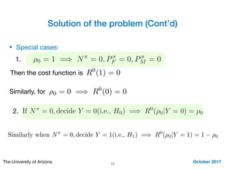
• Special cases:
Then the cost function is
⇢0 = 1 =) N⇡
= 0, P⇡
F = 0, P⇡
M = 0
Similarly, for
R0
(1) = 0
⇢0 = 0 =) R0
(0) = 0
1.
2. If N⇡
= 0, decide Y = 0(i.e., H0) =) R0
(⇢0|Y = 0) = ⇢0
Similarly when N⇡
= 0, decide Y = 1(i.e., H1) =) R0
(⇢0|Y = 1) = 1 ⇢0
Solution of the problem (Cont’d)
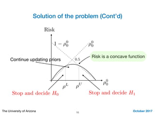
October 2017The University of Arizona 16
⇢0
0
Risk
0.5
1 ⇢0
0 ⇢0
0
Risk is a concave function
⇢L ⇢U
Stop and decide H1Stop and decide H0
Continue updating priors
Solution of the problem (Cont’d)
October 2017The University of Arizona 17
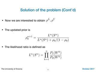
• Now we are interested to obtain ⇢L
, ⇢U
• The updated prior is
⇢n+1
0 =
Ln
(Sn
)
Ln(Sn) + ⇢0/(1 ⇢0)
Ln
(Sn
) =
nY
k=1
P1(Wk
)
P0(Wk)
• The likelihood ratio is defined as
Solution of the problem (Cont’d)
October 2017The University of Arizona 18
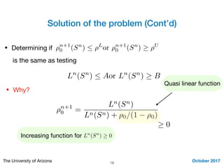
• Determining if
⇢n+1
0 =
Ln
(Sn
)
Ln(Sn) + ⇢0/(1 ⇢0)
⇢n+1
0 (Sn
)  ⇢L
or ⇢n+1
0 (Sn
) ⇢U
is the same as testing
Ln
(Sn
)  Aor Ln
(Sn
) B
• Why?
Quasi linear function
0
Increasing function for Ln
(Sn
) 0
Solution of the problem (Cont’d)
October 2017The University of Arizona 19
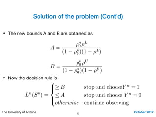
• The new bounds A and B are obtained as
A =
⇢n
0 ⇢L
(1 ⇢n
0 )(1 ⇢L)
B =
⇢n
0 ⇢U
(1 ⇢n
0 )(1 ⇢U )
• Now the decision rule is
Ln
(Sn
) =
8
><
>:
B stop and chooseY n
= 1
 A stop and choose Y n
= 0
otherwise continue observing
Solution of the problem (Cont’d)
October 2017The University of Arizona 20
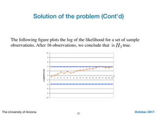
The following figure plots the log of the likelihood for a set of sample
observations. After 16 observations, we conclude that is true.H1
Solution of the problem (Cont’d)
October 2017The University of Arizona 21
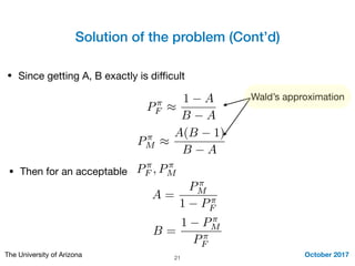
• Since getting A, B exactly is difficult
P⇡
F ⇡
1 A
B A
P⇡
M ⇡
A(B 1)
B A
Wald’s approximation
• Then for an acceptable P⇡
F , P⇡
M
A =
P⇡
M
1 P⇡
F
B =
1 P⇡
M
P⇡
F
Application: Compressive Spectrum Sensing
October 2017The University of Arizona 22
Source: mdpi.com
Fig. Network Model

Stopping Problems

  • 1.
    Stopping Problems Mohamed Seif,PhD student ECE Department October 2017The University of Arizona
  • 2.
    Outline October 2017The Universityof Arizona • Motivation • Preliminaries on Hypothesis Testing • Basic Classic of Stopping Problems • Sequential Probability Ratio Test • Proposed Solution •Application 2
  • 3.
    Motivation October 2017The Universityof Arizona • Stopping problems are a simple but important class of learning problems. •In this problem class, information arrives over time, and we have to choose whether to view the information or stop and make a decision. 3 Event Detector t=0 t=1 t=2 t=3 . . . t=10 Input Signal Sudden Change in observation t=0 t=1 t=2 t=3 . . . t=10 Ideal case: Stop observing and detect the change accurately ! Output Signal
  • 4.
    Preliminaries on HypothesisTesting October 2017The University of Arizona • Consider the following example depicted in the figure. • We have two hypotheses: Fig. Radar System ( H0, if No air fighter H1, if Air fighter exist 4
  • 5.
    Preliminaries on HypothesisTesting (Cont’d) October 2017The University of Arizona • Two sources of error in the process of detecting air fighter: 1. False alarm 2. Mis detection Fig. Radar System =) Prob{ ˆH1|H0} =) Prob{ ˆH0|H1} Pe = P(H0)P( ˆH1|H0) + P(H1)P( ˆH0|H1) • Average probability of error: 5
  • 6.
    Basic Classes ofStopping Problems October 2017The University of Arizona 1. Sequential probability ratio test (Talk focus) 2. Secretary problem 6 We have N candidates, interview K out of N candidates. Then, choose the one who has highest score. Decide as quickly as possible when something is changing.
  • 7.
    Wn = ( ¯µ0 + ✏n , H0 ¯µ1 +✏n , H1 Sequential Probability Ratio Test October 2017The University of Arizona 7 • For example, we may think we are observing data being generated by the sequence • The observed signal at time slot n • Prior probabilities Prob(H0) = ⇢0 = ⇢0 0 Prob(H1) = ⇢1 = ⇢0 1
  • 8.
    Sequential Probability RatioTest October 2017The University of Arizona 8 • After observing W1, update the prior using Baye’s rule as follows ⇢1 0 = P(H0|W1 ) = P(W1 |H0)P(H0) P(W1) = P(W1 |H0)P(H0) ⇢0P(W1|H0) + ⇢0 1P(W1|H1) Similarly, we can update ⇢1 1 ⇢1 1 = P(H1|W1 )
  • 9.
    Example October 2017The Universityof Arizona • Consider the observed signal is drawn from Gaussian distribution, then 9 P(W1 = w|H0) = 1 p 2⇡ exp ✓ 1 2 (w ¯µ0 )2 ◆ • Let, P0(Wn ) = P(Wn = wn |H0)
  • 10.
    Example October 2017The Universityof Arizona 10 ⇢n 0 = ⇢0 Qn k=1 P0(Wk ) ⇢0 Qn k=1 P0(Wk) + ⇢0 1 Qn k=1 P1(Wk) • After n observations, = ⇢0 n (W1 , . . . , Wn ⇢0 + ⇢0 1 n(W1, . . . , Wn) n (W1 , . . . , Wn ) = nY k=1 P0(Wk ) P1(Wk) • Where, )
  • 11.
    Solution of theproblem October 2017The University of Arizona 11 • Denote the set of all experiments as Sn = (W1 , . . . , Wn ) • In the solution / policy , we have two decisions (X⇡ , Y ⇡ )⇡ X⇡ (Sn ) = ( 1, stop and decide 0, continue observing Y ⇡ (Sn ) = ( 1, Decide H1 0, Decide H0
  • 12.
    Solution of theproblem (Cont’d) October 2017The University of Arizona 12 • Two sources of error can happen: 1. False alarm: stop and conclude H1 but the true is the null hypothesis H0 2. Mis detection: we did not pick up any change, i.e., concludeH0 but H1the alternative hypothesis is true P⇡ F = E [Y ⇡ (Sn |H0)] P⇡ M = E [1 Y ⇡ (Sn |H1)] Pe = (1 ⇢0)P⇡ F + ⇢0P⇡ M • Average probability of error:
  • 13.
    Solution of theproblem (Cont’d) October 2017The University of Arizona 13 • Let, N⇡ = min{n|X⇡ (Sn ) = 1} a random variable that depends on our policy , decision function and the observations ⇡ X⇡ (W1 , W2 , . . . , Wn ) • The cost function is defined as follows: U⇡ (c) = Pe + cE(N⇡ ) where is a scaling coefficient.c
  • 14.
    Solution of theproblem (Cont’d) October 2017The University of Arizona 14 • The cost function is decomposed into two conditionals risks r⇡ 0 = P⇡ F + cE(N⇡ |H0) r⇡ 1 = P⇡ M + cE(N⇡ |H1) r⇡ = ⇢0r⇡ 0 + (1 ⇢0)r⇡ 1 • The total cost is in terms of the conditional risks: • Now our objective is R0 (⇢0) = min ⇡ r⇡
  • 15.
    Solution of theproblem (Cont’d) October 2017The University of Arizona 15 • Special cases: Then the cost function is ⇢0 = 1 =) N⇡ = 0, P⇡ F = 0, P⇡ M = 0 Similarly, for R0 (1) = 0 ⇢0 = 0 =) R0 (0) = 0 1. 2. If N⇡ = 0, decide Y = 0(i.e., H0) =) R0 (⇢0|Y = 0) = ⇢0 Similarly when N⇡ = 0, decide Y = 1(i.e., H1) =) R0 (⇢0|Y = 1) = 1 ⇢0
  • 16.
    Solution of theproblem (Cont’d) October 2017The University of Arizona 16 ⇢0 0 Risk 0.5 1 ⇢0 0 ⇢0 0 Risk is a concave function ⇢L ⇢U Stop and decide H1Stop and decide H0 Continue updating priors
  • 17.
    Solution of theproblem (Cont’d) October 2017The University of Arizona 17 • Now we are interested to obtain ⇢L , ⇢U • The updated prior is ⇢n+1 0 = Ln (Sn ) Ln(Sn) + ⇢0/(1 ⇢0) Ln (Sn ) = nY k=1 P1(Wk ) P0(Wk) • The likelihood ratio is defined as
  • 18.
    Solution of theproblem (Cont’d) October 2017The University of Arizona 18 • Determining if ⇢n+1 0 = Ln (Sn ) Ln(Sn) + ⇢0/(1 ⇢0) ⇢n+1 0 (Sn )  ⇢L or ⇢n+1 0 (Sn ) ⇢U is the same as testing Ln (Sn )  Aor Ln (Sn ) B • Why? Quasi linear function 0 Increasing function for Ln (Sn ) 0
  • 19.
    Solution of theproblem (Cont’d) October 2017The University of Arizona 19 • The new bounds A and B are obtained as A = ⇢n 0 ⇢L (1 ⇢n 0 )(1 ⇢L) B = ⇢n 0 ⇢U (1 ⇢n 0 )(1 ⇢U ) • Now the decision rule is Ln (Sn ) = 8 >< >: B stop and chooseY n = 1  A stop and choose Y n = 0 otherwise continue observing
  • 20.
    Solution of theproblem (Cont’d) October 2017The University of Arizona 20 The following figure plots the log of the likelihood for a set of sample observations. After 16 observations, we conclude that is true.H1
  • 21.
    Solution of theproblem (Cont’d) October 2017The University of Arizona 21 • Since getting A, B exactly is difficult P⇡ F ⇡ 1 A B A P⇡ M ⇡ A(B 1) B A Wald’s approximation • Then for an acceptable P⇡ F , P⇡ M A = P⇡ M 1 P⇡ F B = 1 P⇡ M P⇡ F
  • 22.
    Application: Compressive SpectrumSensing October 2017The University of Arizona 22 Source: mdpi.com Fig. Network Model