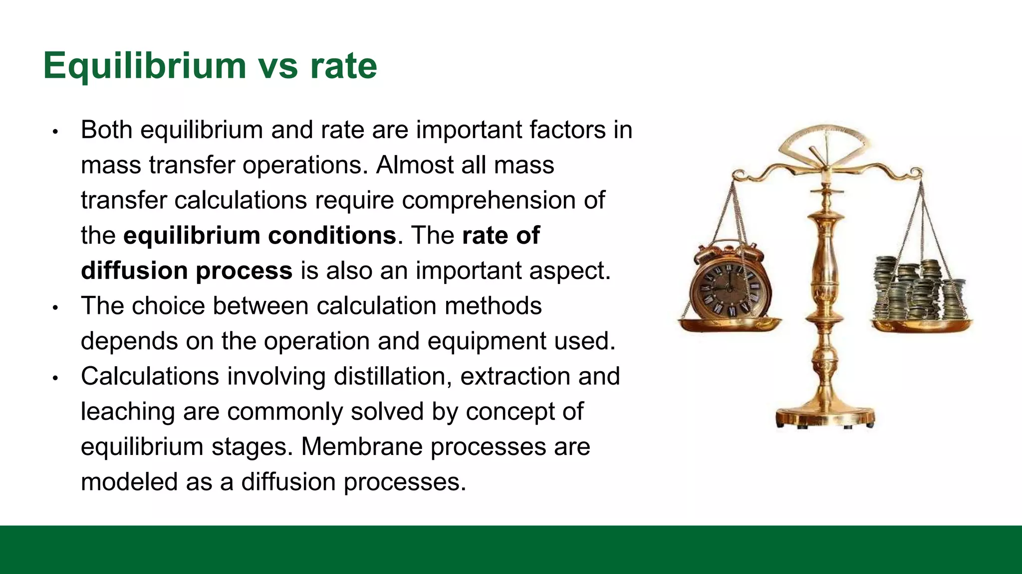
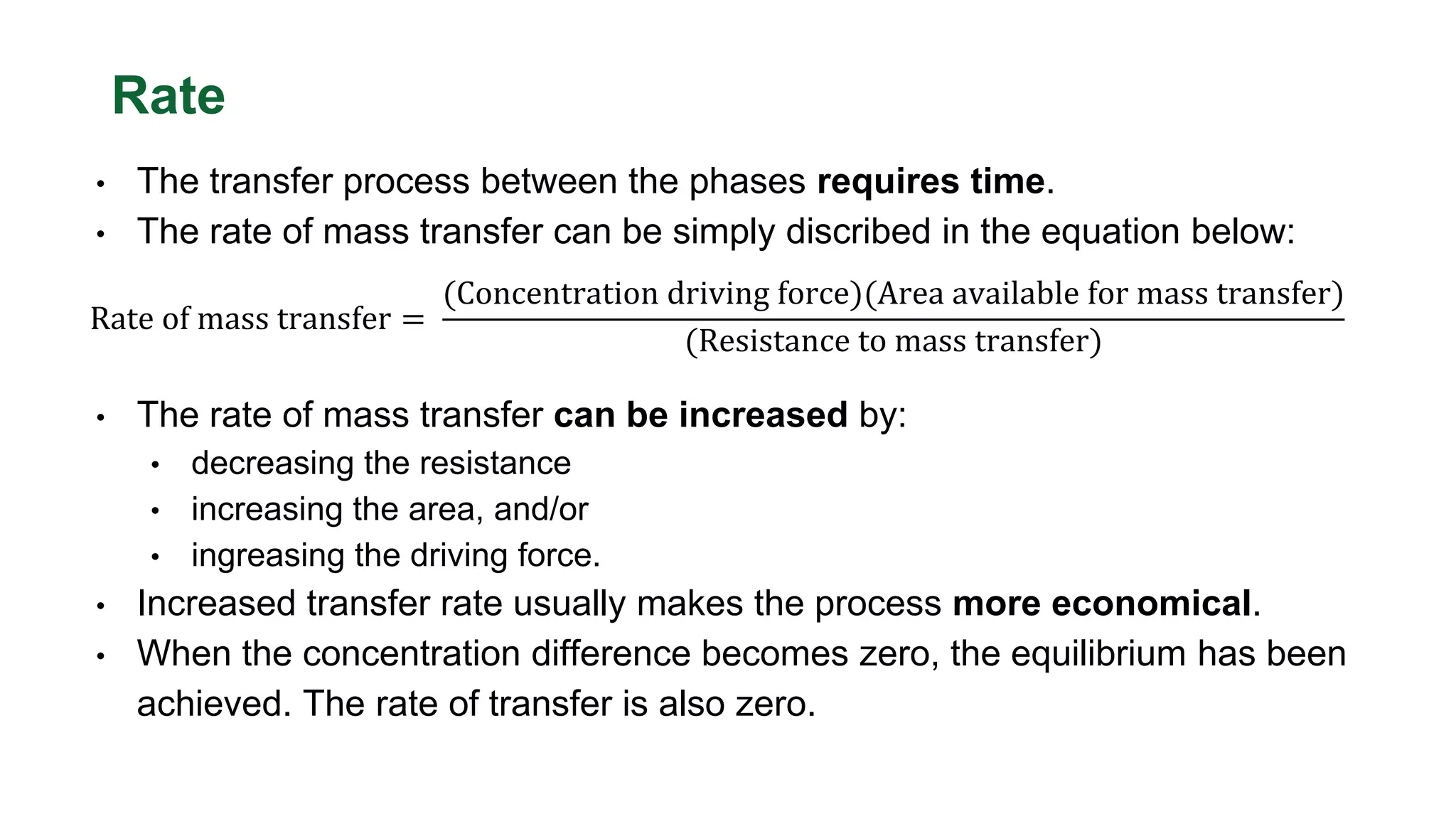
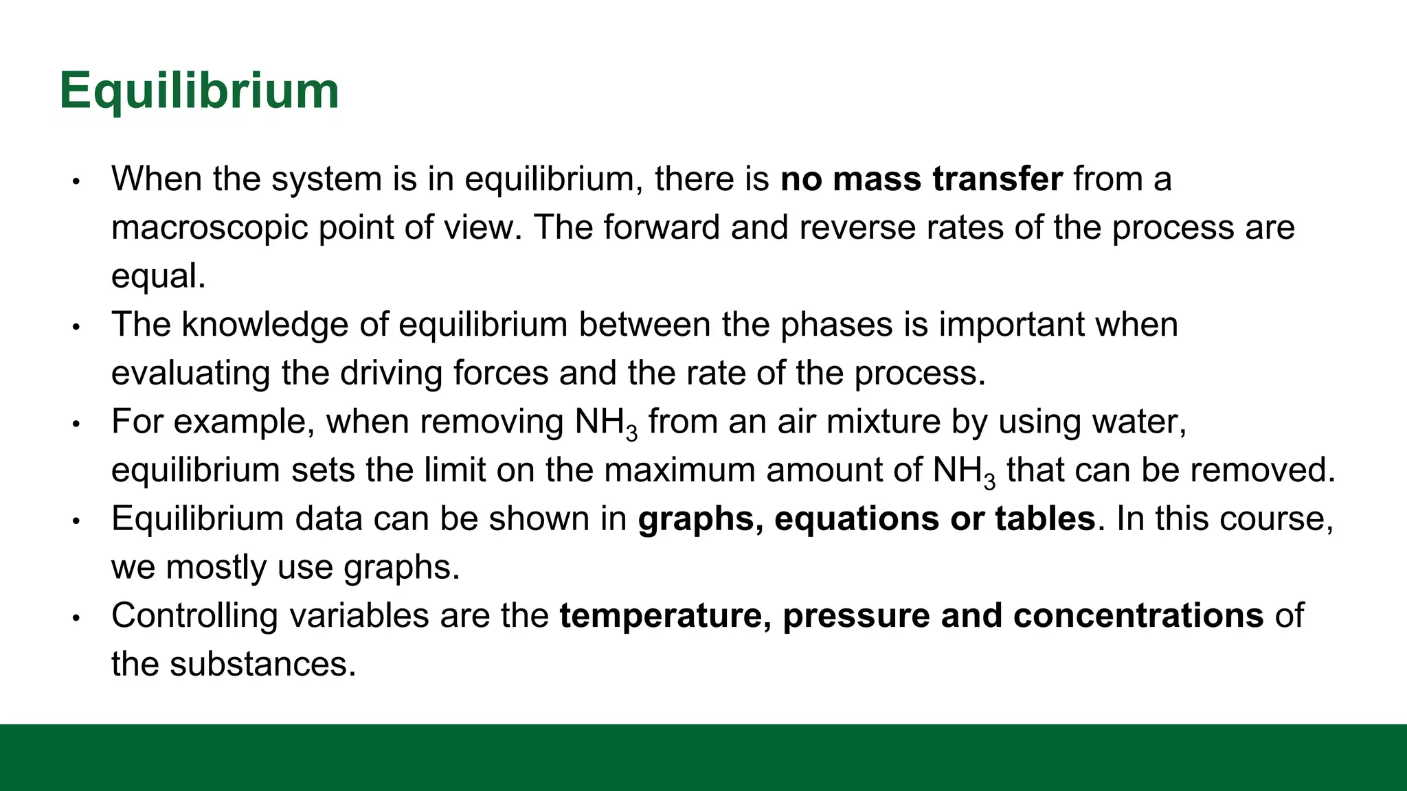
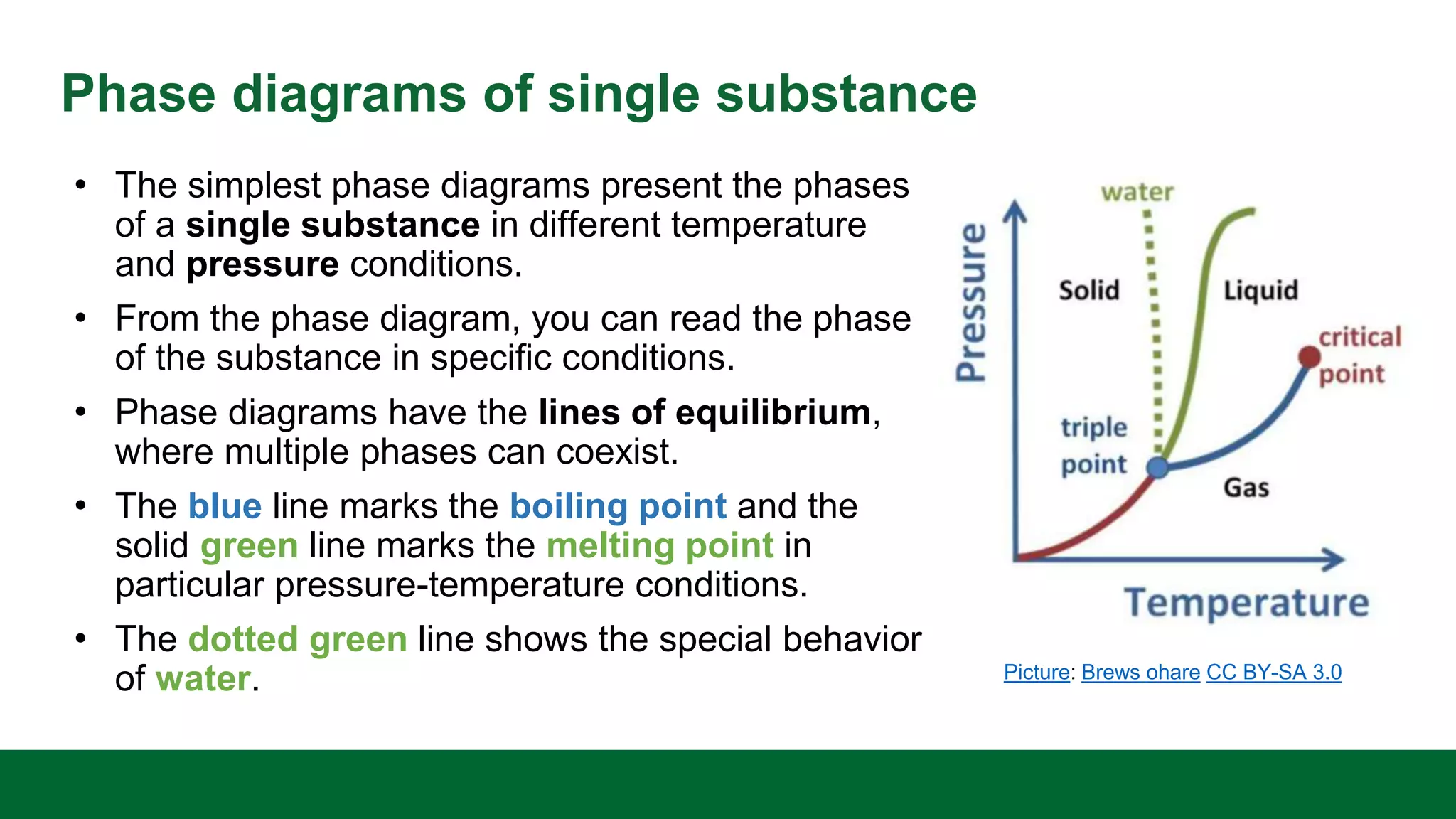
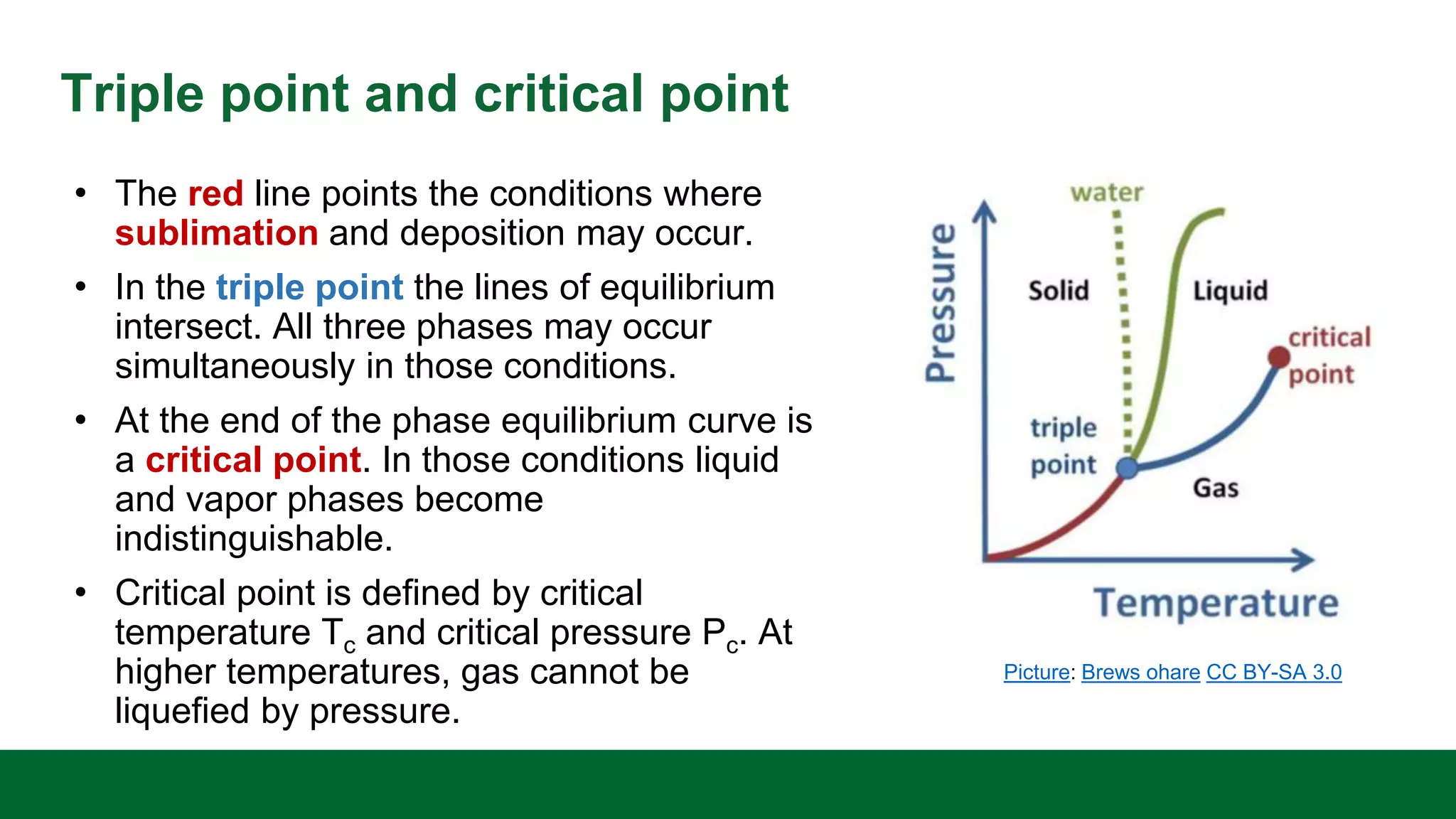
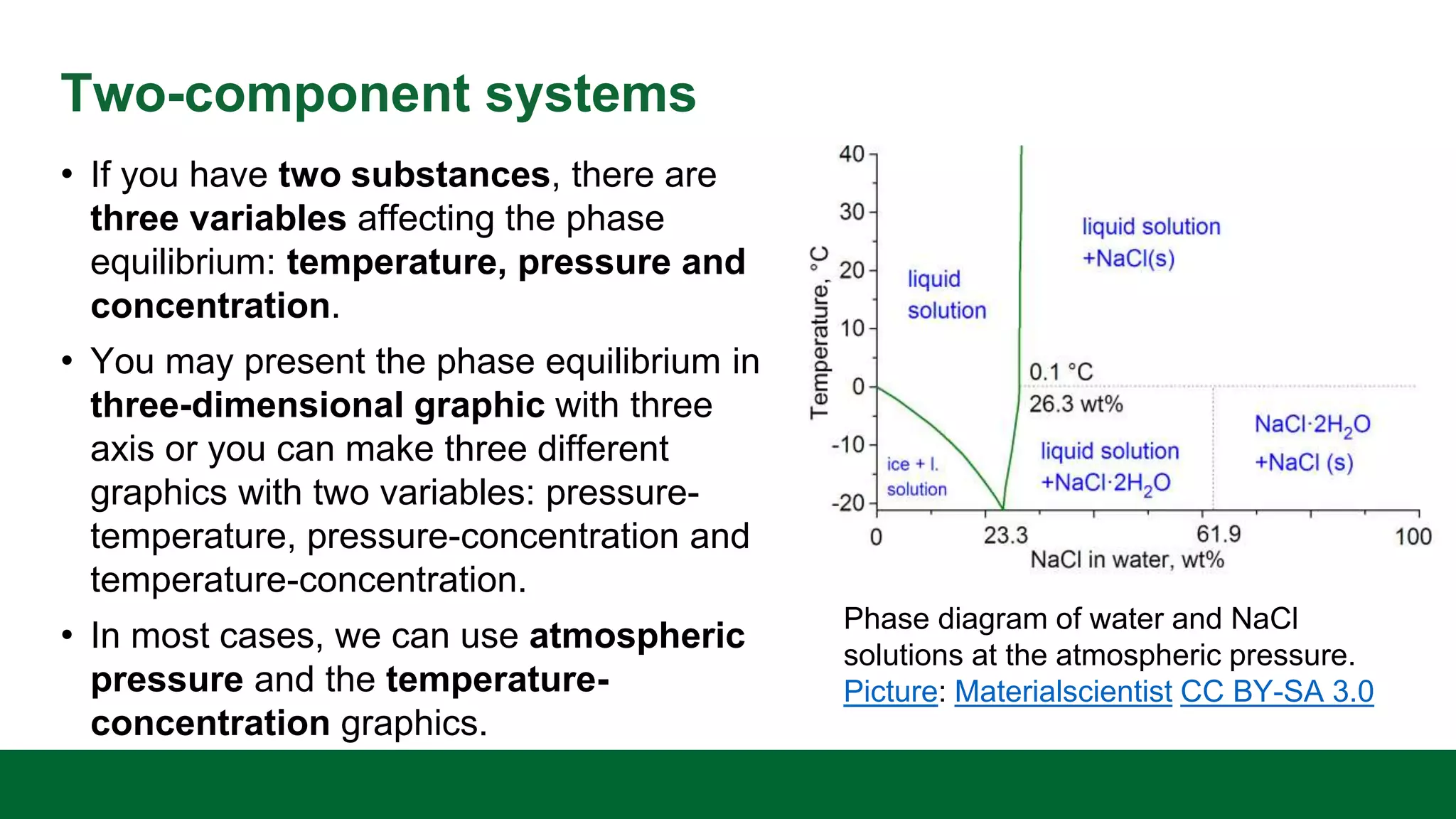
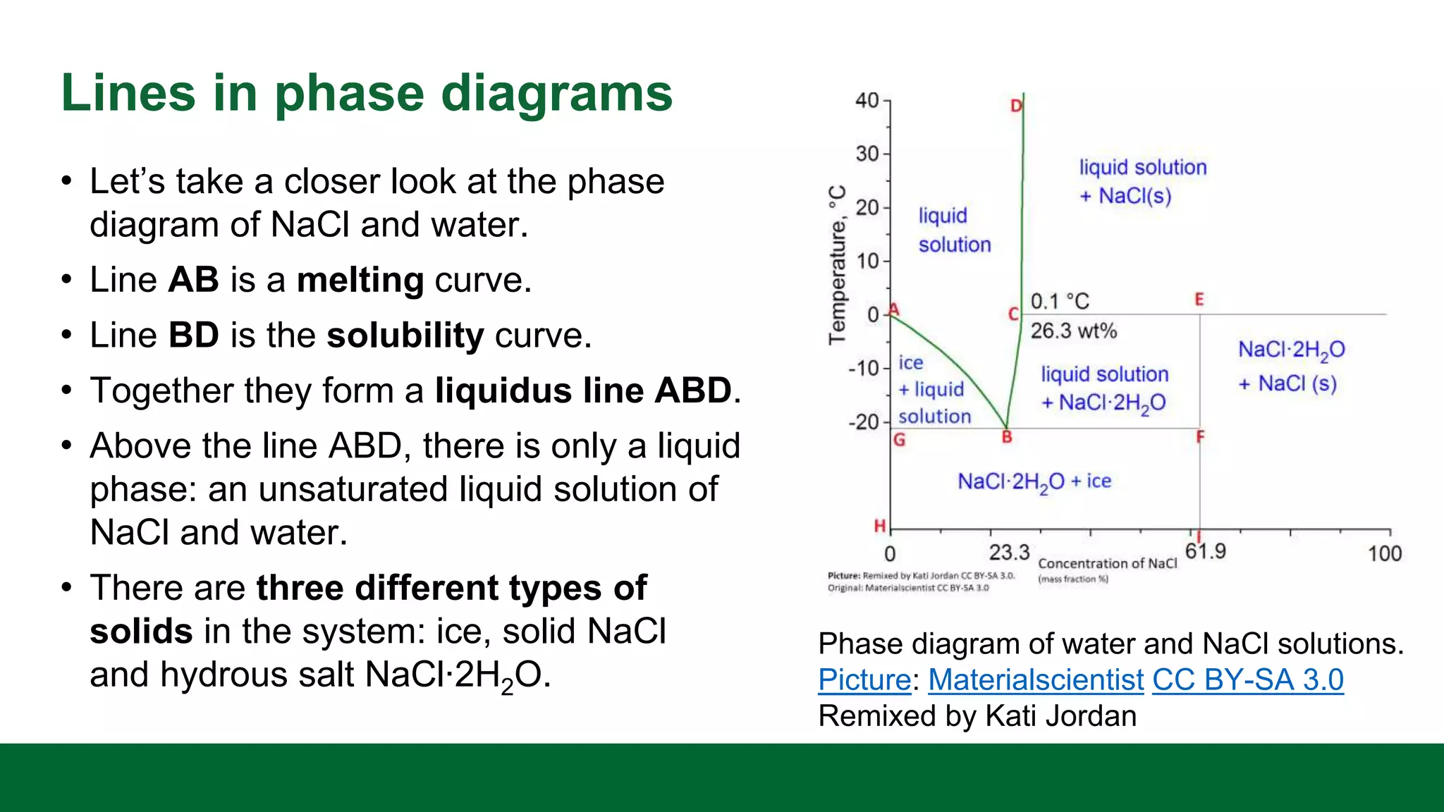
This project has received funding from the European Union’s Horizon 2020
research and innovation programme under grant agreement No 869993.
Rate and
equilibrium
Equilibrium vs rate
• Both equilibrium and rate are important factors in
mass transfer operations. Almost all mass
transfer calculations require comprehension of
the equilibrium conditions. The rate of
diffusion process is also an important aspect.
• The choice between calculation methods
depends on the operation and equipment used.
• Calculations involving distillation, extraction and
leaching are commonly solved by concept of
equilibrium stages. Membrane processes are
modeled as a diffusion processes.
Rate
• The transfer process between the phases requires time.
• The rate of mass transfer can be simply discribed in the equation below:
Rate of mass transfer =
(Concentration driving force)(Area available for mass transfer)
(Resistance to mass transfer)
• The rate of mass transfer can be increased by:
• decreasing the resistance
• increasing the area, and/or
• ingreasing the driving force.
• Increased transfer rate usually makes the process more economical.
• When the concentration difference becomes zero, the equilibrium has been
achieved. The rate of transfer is also zero.
Equilibrium
• When the system is in equilibrium, there is no mass transfer from a
macroscopic point of view. The forward and reverse rates of the process are
equal.
• The knowledge of equilibrium between the phases is important when
evaluating the driving forces and the rate of the process.
• For example, when removing NH3 from an air mixture by using water,
equilibrium sets the limit on the maximum amount of NH3 that can be removed.
• Equilibrium data can be shown in graphs, equations or tables. In this course,
we mostly use graphs.
• Controlling variables are the temperature, pressure and concentrations of
the substances.
Phase diagrams of single substance
• The simplest phase diagrams present the phases
of a single substance in different temperature
and pressure conditions.
• From the phase diagram, you can read the phase
of the substance in specific conditions.
• Phase diagrams have the lines of equilibrium,
where multiple phases can coexist.
• The blue line marks the boiling point and the
solid green line marks the melting point in
particular pressure-temperature conditions.
• The dotted green line shows the special behavior
of water. Picture: Brews ohare CC BY-SA 3.0
Triple point and critical point
• The red line points the conditions where
sublimation and deposition may occur.
• In the triple point the lines of equilibrium
intersect. All three phases may occur
simultaneously in those conditions.
• At the end of the phase equilibrium curve is
a critical point. In those conditions liquid
and vapor phases become
indistinguishable.
• Critical point is defined by critical
temperature Tc and critical pressure Pc. At
higher temperatures, gas cannot be
liquefied by pressure.
Picture: Brews ohare CC BY-SA 3.0
Two-component systems
• If you have two substances, there are
three variables affecting the phase
equilibrium: temperature, pressure and
concentration.
• You may present the phase equilibrium in
three-dimensional graphic with three
axis or you can make three different
graphics with two variables: pressure-
temperature, pressure-concentration and
temperature-concentration.
• In most cases, we can use atmospheric
pressure and the temperature-
concentration graphics.
Phase diagram of water and NaCl
solutions at the atmospheric pressure.
Picture: Materialscientist CC BY-SA 3.0
Lines in phase diagrams
• Let’s take a closer look at the phase
diagram of NaCl and water.
• Line AB is a melting curve.
• Line BD is the solubility curve.
• Together they form a liquidus line ABD.
• Above the line ABD, there is only a liquid
phase: an unsaturated liquid solution of
NaCl and water.
• There are three different types of
solids in the system: ice, solid NaCl
and hydrous salt NaCl∙2H2O.
Phase diagram of water and NaCl solutions.
Picture: Materialscientist CC BY-SA 3.0
Remixed by Kati Jordan
Gibbs phase rule
• J. Willard Gibbs (1839-1903) formulated a phase rule:
F = C – P + 2
F = degrees of freedom
C = components of a system
P = phase (homogeneous parts of a system)
• The phase rule determines how many independent
intensive variables can exist in a specific state of
equilibrium.
• Intensive variables are variables, which do not vary
with the amount of the substance. E.g. temperature,
density and pressure are intensive variables.
• Variables that vary with the amount are called
extensive variables, e.g. mass and volume.
• When we have two phases, F = C.
Two phases and two components
• If we have two components (A and B) and two phases (gas and liquid) in the
distillation process, the degrees of freedom F = C – P + 2 = 2 – 2 + 2 = 2.
• Both components are found in both phases. We have four variables of
interest: temperature, pressure and the mole fractions of component A in the
gas and liquid phases. If the pressure is fixed (e.g. atmospheric pressure),
only one variable can be changed independently. Other two must follow.
• In this case, the equilibrium data can be presented in equilibrium curves:
• temperature-composition diagram or
• by plotting liquid phase mole fraction xA – vapor phase mole fraction yA
• These plots are called Txy-diagram and xy-diagram.
• If we have three components, F = 3. If we then set the temperature and liquid
concentrations xA and xB, the system is defined and all other variables are
determined.
Txy-diagram and xy-diagram
• In the Txy-diagram, there are two lines.
The upper line is called dew point curve and
the other is bubble point curve. In the dew
point, vapor begins to condence. In the bubble
point, liquid begins to vaporize.
• The mole fraction of A can be read from the x-
axis and the temperature from y-axis.
Pictures: Screenshots from the video: https://youtu.be/TkaAl-jaMw8 (LearnChemE)
• The xy-diagram can be
drawn from the information of
Txy-diagram. The green line
is the equilibrium curve.
This project has received funding from the European Union’s Horizon 2020
research and innovation programme under grant agreement No 869993.
References
McCabe, W. L., Smith, J. C. & Harriott, P. 2005. Unit operations of chemical engineering.
7th ed. Boston: McGraw-Hill, pp. 521-525.
Theodore, L. & Ricci, F. 2010. Mass Transfer Operations for the Practicing Engineer. John
Wiley & Sons, Inc, pp. 37-72.
Videos:
• Txy-diagram and xy-diagram: https://youtu.be/TkaAl-jaMw8
• Phase diagrams of binary solutions: https://youtu.be/SPrybbPdVDQ
• Gibbs phase rule: https://youtu.be/_XYdPIqYXRU
• Intro to phase diagrams: https://youtu.be/MJoYwtX_zFA

Rate and equilibrium in mass transfer processes

  • 1.
    This project hasreceived funding from the European Union’s Horizon 2020 research and innovation programme under grant agreement No 869993. Rate and equilibrium
  • 2.
    Equilibrium vs rate •Both equilibrium and rate are important factors in mass transfer operations. Almost all mass transfer calculations require comprehension of the equilibrium conditions. The rate of diffusion process is also an important aspect. • The choice between calculation methods depends on the operation and equipment used. • Calculations involving distillation, extraction and leaching are commonly solved by concept of equilibrium stages. Membrane processes are modeled as a diffusion processes.
  • 3.
    Rate • The transferprocess between the phases requires time. • The rate of mass transfer can be simply discribed in the equation below: Rate of mass transfer = (Concentration driving force)(Area available for mass transfer) (Resistance to mass transfer) • The rate of mass transfer can be increased by: • decreasing the resistance • increasing the area, and/or • ingreasing the driving force. • Increased transfer rate usually makes the process more economical. • When the concentration difference becomes zero, the equilibrium has been achieved. The rate of transfer is also zero.
  • 4.
    Equilibrium • When thesystem is in equilibrium, there is no mass transfer from a macroscopic point of view. The forward and reverse rates of the process are equal. • The knowledge of equilibrium between the phases is important when evaluating the driving forces and the rate of the process. • For example, when removing NH3 from an air mixture by using water, equilibrium sets the limit on the maximum amount of NH3 that can be removed. • Equilibrium data can be shown in graphs, equations or tables. In this course, we mostly use graphs. • Controlling variables are the temperature, pressure and concentrations of the substances.
  • 5.
    Phase diagrams ofsingle substance • The simplest phase diagrams present the phases of a single substance in different temperature and pressure conditions. • From the phase diagram, you can read the phase of the substance in specific conditions. • Phase diagrams have the lines of equilibrium, where multiple phases can coexist. • The blue line marks the boiling point and the solid green line marks the melting point in particular pressure-temperature conditions. • The dotted green line shows the special behavior of water. Picture: Brews ohare CC BY-SA 3.0
  • 6.
    Triple point andcritical point • The red line points the conditions where sublimation and deposition may occur. • In the triple point the lines of equilibrium intersect. All three phases may occur simultaneously in those conditions. • At the end of the phase equilibrium curve is a critical point. In those conditions liquid and vapor phases become indistinguishable. • Critical point is defined by critical temperature Tc and critical pressure Pc. At higher temperatures, gas cannot be liquefied by pressure. Picture: Brews ohare CC BY-SA 3.0
  • 7.
    Two-component systems • Ifyou have two substances, there are three variables affecting the phase equilibrium: temperature, pressure and concentration. • You may present the phase equilibrium in three-dimensional graphic with three axis or you can make three different graphics with two variables: pressure- temperature, pressure-concentration and temperature-concentration. • In most cases, we can use atmospheric pressure and the temperature- concentration graphics. Phase diagram of water and NaCl solutions at the atmospheric pressure. Picture: Materialscientist CC BY-SA 3.0
  • 8.
    Lines in phasediagrams • Let’s take a closer look at the phase diagram of NaCl and water. • Line AB is a melting curve. • Line BD is the solubility curve. • Together they form a liquidus line ABD. • Above the line ABD, there is only a liquid phase: an unsaturated liquid solution of NaCl and water. • There are three different types of solids in the system: ice, solid NaCl and hydrous salt NaCl∙2H2O. Phase diagram of water and NaCl solutions. Picture: Materialscientist CC BY-SA 3.0 Remixed by Kati Jordan
  • 9.
    Gibbs phase rule •J. Willard Gibbs (1839-1903) formulated a phase rule: F = C – P + 2 F = degrees of freedom C = components of a system P = phase (homogeneous parts of a system) • The phase rule determines how many independent intensive variables can exist in a specific state of equilibrium. • Intensive variables are variables, which do not vary with the amount of the substance. E.g. temperature, density and pressure are intensive variables. • Variables that vary with the amount are called extensive variables, e.g. mass and volume. • When we have two phases, F = C.
  • 10.
    Two phases andtwo components • If we have two components (A and B) and two phases (gas and liquid) in the distillation process, the degrees of freedom F = C – P + 2 = 2 – 2 + 2 = 2. • Both components are found in both phases. We have four variables of interest: temperature, pressure and the mole fractions of component A in the gas and liquid phases. If the pressure is fixed (e.g. atmospheric pressure), only one variable can be changed independently. Other two must follow. • In this case, the equilibrium data can be presented in equilibrium curves: • temperature-composition diagram or • by plotting liquid phase mole fraction xA – vapor phase mole fraction yA • These plots are called Txy-diagram and xy-diagram. • If we have three components, F = 3. If we then set the temperature and liquid concentrations xA and xB, the system is defined and all other variables are determined.
  • 11.
    Txy-diagram and xy-diagram •In the Txy-diagram, there are two lines. The upper line is called dew point curve and the other is bubble point curve. In the dew point, vapor begins to condence. In the bubble point, liquid begins to vaporize. • The mole fraction of A can be read from the x- axis and the temperature from y-axis. Pictures: Screenshots from the video: https://youtu.be/TkaAl-jaMw8 (LearnChemE) • The xy-diagram can be drawn from the information of Txy-diagram. The green line is the equilibrium curve.
  • 12.
    This project hasreceived funding from the European Union’s Horizon 2020 research and innovation programme under grant agreement No 869993. References McCabe, W. L., Smith, J. C. & Harriott, P. 2005. Unit operations of chemical engineering. 7th ed. Boston: McGraw-Hill, pp. 521-525. Theodore, L. & Ricci, F. 2010. Mass Transfer Operations for the Practicing Engineer. John Wiley & Sons, Inc, pp. 37-72. Videos: • Txy-diagram and xy-diagram: https://youtu.be/TkaAl-jaMw8 • Phase diagrams of binary solutions: https://youtu.be/SPrybbPdVDQ • Gibbs phase rule: https://youtu.be/_XYdPIqYXRU • Intro to phase diagrams: https://youtu.be/MJoYwtX_zFA