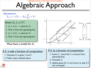
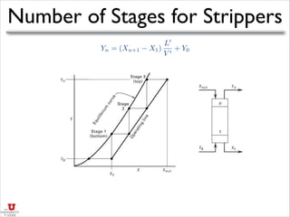
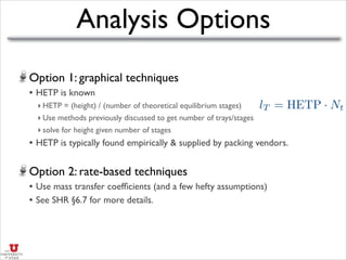
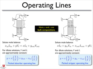
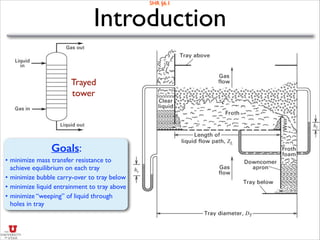
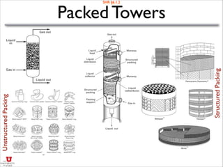
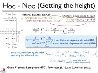
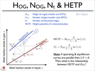
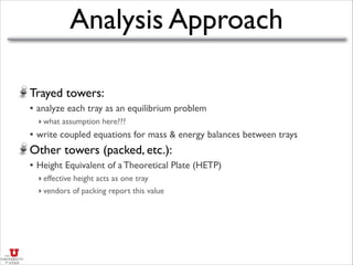
- This document describes absorption and stripping processes using packed columns and graphical methods. - It discusses operating lines, height of transfer units (HOG), number of transfer units (NOG), and how to calculate the height equivalent of a theoretical plate (HETP) for a packed column given mass transfer coefficients, flow rates, and equilibrium data. - An example is provided to calculate the HETP for a specific packed column based on the mass transfer coefficients, flow rates, and equilibrium constant given.

1. Absorption & Stripping
• Introduction
• Graphical Methods
• Packed Towers
SHR Chapter 6

2. Introduction
Trayed
tower
Goals:
• minimize mass transfer resistance to
achieve equilibrium on each tray
• minimize bubble carry-over to tray below
• minimize liquid entrainment to tray above
• minimize “weeping” of liquid through
holes in tray
SHR §6.1

3. Types of Trays
perforated valve cap bubble cap

4. Regimes in a Trayed Tower
“Spray”
gas phase is continuous
(low liquid depths, high gas
flow rates)
“Froth”
gas passes through liquid as
jets or a series of bubbles
“Emulsion”
!
“Bubble”
low gas flow rates -
swarms of bubbles
“Cellular Foam”
(think blowing bubbles
in chocolate milk)
SHR §6.1.1

5. Packed Towers
StructuredPacking
UnstructuredPacking
SHR §6.1.2

6. Other Configurations
Spray tower
• very low pressure drop
• use for absorption only when
solute is highly soluble in the
liquid (e.g. SO2 in flue gas)
Bubble column
• absorption
• high pressure drop
• use when solute is poorly
soluble in liquid
• use when slow chemical
reactions occur that require
long residence time
Centrifugal contactor
• short residence time
• compact
SHR §6.1.3

7. Heuristics & Design Considerations
Trayed towers
• “reliable” design
• low liquid velocities
• liquid phase (the continuous phase) is typically mass-transfer limiting
Unstructured Packed towers
• corrosive environments
• small towers (<2 ft diameter, <20 ft tall)
• when foaming problems tend to occur
• gas phase (continuous phase) is typically mass-transfer limiting
Structured packed towers
• (expensive!)
• retrofit when trying to get more efficiency
• low pressure drop
• gas phase (continuous phase) is typically mass-transfer limiting

8. Analysis Approach
Trayed towers:
• analyze each tray as an equilibrium problem
‣ what assumption here???
• write coupled equations for mass & energy balances between trays
Other towers (packed, etc.):
• Height Equivalent of a Theoretical Plate (HETP)
‣ effective height acts as one tray
‣ vendors of packing report this value

9. Graphical Methods
SHR §6.3

10. Some Terminology
Stripper
Solute enters in liquid.
Stripping agent enters
bottom of column.
L′
Molar flow rate of solute-free liquid
V′
Molar flow rate of solute-free gas
x
mole fraction of solute in liquid
y
mole fraction of solute in gas
X
mole ratio of solute to solute-free liquid
Y
mole ratio of solute to solute-free gas
Assume that only solute is transferred from
one phase to another (no vaporization of
liquid or condensation of gas carriers).
What does XL′ and
YV′ represent?
X =
x
1 x
Y =
y
1 y
Absorber
Solute enters in gas.
Liquid absorbent enters
from top of column.
Note different
tray ordering
convention...
Stage "i"
Xi
Xi-1 Yi
Yi+1
For the absorber:
Ki =
yi
xi
=
Yi/(1+Yi)
Xi/(1+Xi)
Streams leaving the tray are
assumed to be in equilibrium

11. Mole Balances & Operating Lines
Solute balance around arbitrary # of trays
in the “top” section of the absorber:
X0L0
+ Yn+1V 0
= XnL0
+ Y1V 0
solute flow rate in solute flow rate out
Yn+1 = (Xn X0)
L0
V 0
+ Y1
L0
V 0 = “slope” of operating line
(absorber)
(stripper)
What happens as ?L0
/V 0
! 1
Absorber
Solute enters in gas.
Liquid absorbent enters
from top of column.
We know
these.
What happens as gets small?L0
/V 0
Yn = (Xn+1 X1)
L0
V 0
+ Y0
SHR §6.3.2
For an absorber, we typically know
YN+1, X0 and Vʹ. Therefore, we get
to choose Lʹ to achieve desired Y1.
design
variable

12. Absorber: Minimum Flow Rate
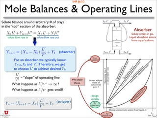
Yn+1 = (Xn X0)
L0
V 0
+ Y1
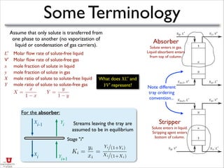
Absorber
Solute enters in gas.
Liquid absorbent enters
from top of column.
L0
=
V 0
(YN+1 Y1)
XN X0
Over the whole tower (n=N):
L′min corresponds to equilibrium
with XN and YN+1.
KN =
yN+1
xN
=
YN+1/(1+YN+1)
XN/(1+XN )
For dilute solutes (Y ≈ y and X ≈ x):
If X0 ≈ 0 then:
L0
min = V 0
✓
yN+1 y1
yN+1/KN x0
◆
Corresponding
equation for a
stripper:
L0
min =
V 0
(YN+1 Y1)
YN+1/[YN+1(KN 1)+KN ] X0
As V′ ↑, L′min↑.
SHR §6.3.3
Why are these in equilibrium?
L0
min = V 0
KN · (fraction absorbed)
V 0
min =
L0
KN
· (fraction stripped)
This is the “best” we can achieve
given the inlet constraints.

13. Examples
Given: feed stream
composition & flow
rates, recovery (Y1)
Find: XN.
Given: feed stream
composition & flow rates,
solvent loading (XN)
Find: Y1.
Given: feed stream composition, gas flow
rate, solvent loading (XN), and recovery (Y1),
Find: solvent flow rate.
Yn+1 = (Xn X0)
L0
V 0
+ Y1
X
Y
XNX0
YN+1
Y1
Y
=
KX
L'
V'
X
Y
XNX0
YN+1
Y1
Y
=
KX
L'
V'
X
Y
XNX0
YN+1
Y1
Y
=
KX
L'
V'

14. Number of “Equilibrium” Stages
SHR §6.3.4
1. Locate the point for the solvent feed
(X0) and desired Y1 on the graph.
2. Determine operating line from Vʹ and Lʹ.
3. March off to determine the stages
(assuming each stage is in equilibrium)
Stage "i"
Xi
X
i-1
Y
i
Yi+1
For the absorber:
•Streams leaving the tray are
assumed to be in equilibrium
•Streams passing one another
are on the operating line.
Yn+1 = (Xn X0)
L0
V 0
+ Y1
equilibrium
relates Yi
and Xi.
Operating line:
What happens to the
number of stages as Lʹ/Vʹ
approaches ∞ or its
minimum?

15. Algebraic Approach
Yn+1 = (Xn X0)
L0
V 0
+ Y1
Operating line:
Given: X0, Y1, Lʹ/Vʹ,
1. K1 = Y1/X1 → solve for X1.
2. Find Y2 from the operating line.
3. K2 = Y2/X2 → solve for X2.
4. Find Y3 from the operating line.
⋮
Must have a model for Ki.
If Ki is not a function of composition:
1. Calculate Ki at given T and P.
2. Follow steps outlined above.
If Ki is a function of composition:
1. Guess Xi. (note that Yi is known from
operating line).
2. Calculate Ki.
3. Update guess for Xi and return to step 2 if
not converged.
SHR §6.4 presents an alternative to this formulation.

16. Number of Stages for Strippers
Yn = (Xn+1 X1)
L0
V 0
+ Y0

17. Stage Efficiency
Complex function of:
• tray design/geometry
• fluid dynamics on trays
Typically less than 50%
efficient (10%-50%)
• trays are not at equilibrium!
• more viscous liquids typically lead
to lower efficiencies (inhibit mass
transfer)
log Eo = 1.597 0.199 log
✓
KMLµL
⇢L
◆
0.0896

log
✓
KMLµL
⇢L
◆ 2
Empirical correlation for stage efficiency
Data over a wide range of column diameters,
pressures, temperatures and liquid viscosities.
Eo ⌘
Nt
Na
# theoretical
(equilibrium) stages
# actual stages
Other (less empirical) methods
exist - see SHR §6.5.4.

18. Packed Columns
SHR §6.7
SHR §6.7

19. Analysis Options
Option 1: graphical techniques
• HETP is known
‣ HETP = (height) / (number of theoretical equilibrium stages)
‣ Use methods previously discussed to get number of trays/stages
‣ solve for height given number of stages
• HETP is typically found empirically & supplied by packing vendors.
!
Option 2: rate-based techniques
• Use mass transfer coefficients (and a few hefty assumptions)
• See SHR §6.7 for more details.
lT = HETP · Nt

20. Operating Lines
xinLin + yV` = xL` + youtVout
y = x
✓
L
V
◆
+ yout xin
✓
L
V
◆
Solute mole balance:
For dilute solutions, V and L
are approximately constant:
Packed absorber operating line
y = x
✓
L
V
◆
+ yin xout
✓
L
V
◆
Solute mole balance:
For dilute solutions, V and L
are approximately constant:
xL` + yinVin = xoutLout + yV`
Packed stripper operating line
Here, x and y are
bulk compositions.

21. Finite-Rate Mass Transfer
(Back to Two-Film Theory)
Often we don’t know the surface area for
mass transfer from all of the packing.
r = mass transfer rate per
unit volume,
a = surface area per unit
volume of packing
mol/(m3
·s)
r = Ja = kya(y yI)
= kxa(xI x)
y = yI
kxa
kya
(x xI)
relative resistance of
mass transfer between
the two phases
Gas Interface Liquid
liquid film
composition
gas filmcomposition yI or pI
xI or cI
bulk liquid
composition
bulk gas
composition
y or p
x or c
x*
y*
r = Kya (y y⇤
) = Kxa (x⇤
x)
Overall mass transfer coefficient approach:
1
Kya
=
1
kya
+
K
kxa
1
Kxa
=
1
kxa
+
1
Kkya
J = ky(y yI)

22. y = yI
kxa
kya
(x xI)AB line:
Making Connections...
y = x
✓
L
V
◆
+ yout xin
✓
L
V
◆
Applicable
for small x, y.
Gas Interface Liquid
liquid film
composition
gas filmcomposition yI or pI
xI or cI
bulk liquid
composition
bulk gas
composition
y or p
x or c
x*
y*
Operating line:
Mole fraction solute in liquid, x
Molefractionsoluteingas,y
Equilibrium
curve, y=KxO
perating
line
A
B
CF
E
D
(y⇤
, x)
(yI, xI)
(y, x⇤
)
(y, x) y
=
x
✓ L
V
◆ +
yout
xin
✓ L
V
◆
NA = Kx(x⇤
A xAb
)
= Ky(yAb
y⇤
A)
1
Kx
=
1
KAky
+
1
kx
1
Ky
=
1
ky
+
KA
kx
x⇤
A =
yAb
KA
Liquid mole fraction
Gas mole fraction y⇤
A = xAb
KA
From Mass-transfer notes on two-film theory:
What do AE and
AF represent?
comes from
equating “r” in
bulk and interface.

23. HOG - NOG (Getting the height)
Material balance over dl:
Change in gas phase: V (y + dy) - Vy
Transfer to liquid phase: Kya (y - y*) S dl
V dy = Kya(y y⇤
)S dl
KyaS
V
Z lT
0
dl =
KyaSlT
V
=
Z yin
yout
dy
y y⇤
lT =
V
KyaS
| {z }
HOG
Z yin
yout
dy
y y⇤
| {z }
NOG
HOG:
Height of a (gas) transfer unit (HTU)
NOG:
Number of (gas) transfer units (NTU)
For y* = Kx (constant K), and linear
operating line (dilute solute),
A = L/(KV )
Given Ky (overall gas-phase MTC), flow rates (L/V), and K, we can get lT.
NOG =
A
A 1
ln
⇢
(A 1) (yin Kxin)
A (yout Kxin)
+ 1/A
A - “Absorption factor”
see SHR §5.4.1 for derivation of A.
What leaves the gas, goes to the liquid:

24. HOG, NOG, Nt & HETP
HOG:
Height of a (gas) transfer unit (HTU)
NOG:
Number of (gas) transfer units (NTU)
Nt:
Number of theoretical stages
HETP:
Height-equivalent of a theoretical plate
A = L/(KV )
Nt = NOG
A
1 A
ln (1/A)
Mole fraction solute in liquid, x
Molefractionsoluteingas,y
Equilibrium
curve, y=KxO
perating
line
A
B
CF
E
D
(y⇤
, x)
(yI, xI)
(y, x⇤
)
(y, x) y
=
x
✓ L
V
◆ +
yout
xin
✓ L
V
◆
Note: if operating & equilibrium
curves are parallel then L/V = K.
Then what is the relationship
between HETP and HOG?
HETP = HOG
A
1 A
ln (1/A)

25. Example
L, xin V, yout
V, yin L, xout
3,500 lbmol/hr
water
2,500 lbmol/hr
2% ethylene oxide in
inert gas
T=30 ºC
P=20 atm
!
• Two 12’ sections of 1.5” metal Pall ring packing
• 4’ diameter column
• K = 0.85 for ethylene-oxide
• kya = 200 lbmol/(h-ft3)
• kxa = 165 lbmol/(h-ft3)
Find HETP for this packing.
HOG =
V
KyaS
HETP = HOG
A
1 A
ln (1/A) A = L/(KV )
1
Kya
=
1
kya
+
K
kxa