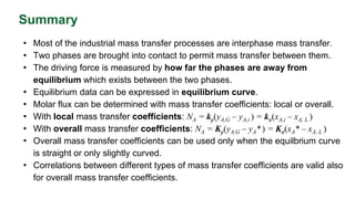
This project has received funding from the European Union’s Horizon 2020
research and innovation programme under grant agreement No 869993.
Interphase
mass transfer
Interphase mass transfer
• Molecular diffusion and convective mass transfer concerned only the mass
transfer within a single phase.
• In practical applications, there are usually two insoluble phases brought
into contact to permit mass transfer between them.
• In one-phase system, the rate of diffusion is dependent upon concentration
differences within the phase.
• In two-phase system, the driving force is measured by how far the phases
are away from equilibrium which exists between the two phases.
• When the equilibrium is achieved, the net rate of diffusion will fall to zero.
• Molecules continue to transfer back and forward, but concentrations within
each phase no longer change.
Equilibrium
• Let’s consider an example where ammonia (NH3) is
dissolved from ammonia-air mixture into liquid water.
• Fixed amount of water and ammonia-air mixture are
placed in a closed container at constant temperature
and pressure. Ammonia is very soluble in water and
it starts to transfer into water through the interface.
• Part of ammonia molecules escapes back into the
gas. This continues until the rates are equal and net
transfer falls to zero.
• With time, concentrations throughout each phase
become uniform by diffusion. Equilibrium is
achieved.
yA
xA
xA = Mole fraction of
ammonia in the liquid
yA = Mole fraction of
ammonia in the gas
Equilibrium-distribution curve
• If additional ammonia is injected into
the container, a new set of equilibrium
concentrations will be eventually
established. Concentrations in both
phases (xA and yA) are now higher.
• This equilibrium data can be
presented in equilibrium curve: mole
fraction in the liquid on the x-axis and
mole fraction in the gas on the y-axis.
• Pressure and temperature are fixed.
Picture: Benitez 2016, 160.
Diffusion between phases
• Industrial mass transfer operations are usually
carried out under steady-state conditions. It
means that the concentrations do not vary with
time at any position in the apparatus.
• Let’s continue with the gas absorption example.
Ammonia-air mixture is feeded from the bottom
of the column and water is feeded from top.
• Water absorbs the ammonia as it flows
downward and the concentration of ammonia
in gas decreases as the gas flows upward.
• The concentrations at any particular point in
the column do not change with time.
Simplified absorption column
Picture by Jocelynskim - CC BY-SA 4.0
remixed by Kati Jordan
Two-resistance film theory
• Interphase mass transfer can be
divided into three steps:
1. Transfer of mass from bulk flow of
one phase to the interfacial surface
2. Transfer of mass across interface
into the second phase
3. Transfer of mass to the bulk flow of
the second phase
• Situation in a particular level of the
column can be visualized graphically.
• Concentrations xA,i and yA,i are the
equilibrium values from the
equilibrium curve. Picture: Benitez 2016, 165.
Mass transfer coefficients and slope
• Let's put those values into the equilibrium
diagram.
• Point P represents the concentrations in the
bulk phases (gas and liquid), and point M
presents the values in the interphase.
• Because we have a steady-state system, molar
fluxes of ammonia are equal in both directions:
NA = ky(yA,G – yA,i ) = kx(xA,i – xA, L )
• ky = local mass transfer coefficient in gas phase
kx= local mass transfer coefficient in liquid
yA,G and xA,L are bulk mole fractions
• yA,i and xA,i the mole fractions in the interphase
Slope of the line PM can be
determined by the local mass
transfer coefficients.
Picture: Benitez 2016, 166.
Overall mass transfer coefficients
• It is usually hard to determine the
interphase concentrations yA,i and xA,i.
• Overall mass transfer coefficients can be
determined by the equilibrium
concentrations yA* and xA* with
respective to bulk concentrations.
NA = Ky(yA,G – yA* ) = Kx(xA* – xA, L )
• Overall mass transfer coefficients are
marked with upper case K.
• These overall coefficients are exactly
valid only in those situations, when the
equilibrium-distribution line is straight.
Picture: Benitez 2016, 167.
Correlations between mass transfer coefficients
• When the equilibrium relation is linear, the relations between gas and liquid
phase concentrations can be presented with proportionality constant m.
• yA,i = mxA,i yA* = mxA,L yA,G = mxA*
• On these circumstances, the following equations are valid:
• Many values for mass transfer coefficients have been determined by
experimental studies. Values can be converted to other forms.
• Correlations between different types of mass transfer coefficients presented
in Chapter 2.3 Convective mass transfer are valid also here. For example:
1
𝐾𝑦
=
1
𝑘𝑦
+
𝑚
𝑘𝑥
1
𝐾𝑥
=
1
𝑚𝑘𝑦
+
1
𝑘𝑥
𝐾𝑦 = 𝑃𝐾𝐺 =
𝑃𝐾𝐶
𝑅𝑇
Example
• Absorption of ammonia by water in a wetted-wall column.
Temperature T = 300 K and pressure P = 1 atm = 101.325 kPa
Proportionality constant m = 1.64 at those circumstances and dilute solutions
At one point in the column xA,L = 0.00115 and yA,G = 0.08
Experimental value of KG = 2.75 ∙ 10-6 kmol/(m2∙s∙kPa)
Calculate the molar flux NA.
Solution: NA = Ky(yA,G – yA* )
yA* = mxA,L = 1.64 ∙ 0.00115 = 1.886 ∙ 10-3
𝑁𝐴 = 2.7864 … ∙ 10−4
kmol
m2 ∙ s
∙ 0.08−1.886 ∙ 10−3 ≈ 2.18 ∙ 10−5
kmol
m2 ∙ s
𝐾𝑦 = 𝑃𝐾𝐺 = 101.325 kPa ∙ 2.75 ∙ 10−6
kmol
m2 ∙ s ∙ kPa
= 2.7864 … ∙ 10−4
kmol
m2 ∙ s
Summary
• Most of the industrial mass transfer processes are interphase mass transfer.
• Two phases are brought into contact to permit mass transfer between them.
• The driving force is measured by how far the phases are away from
equilibrium which exists between the two phases.
• Equilibrium data can be expressed in equilibrium curve.
• Molar flux can be determined with mass transfer coefficients: local or overall.
• With local mass transfer coefficients: NA = ky(yA,G – yA,i ) = kx(xA,i – xA, L )
• With overall mass transfer coefficients: NA = Ky(yA,G – yA* ) = Kx(xA* – xA, L )
• Overall mass transfer coefficients can be used only when the equilbrium curve
is straight or only slightly curved.
• Correlations between different types of mass transfer coefficients are valid also
for overall mass transfer coefficients.
This project has received funding from the European Union’s Horizon 2020
research and innovation programme under grant agreement No 869993.
References
Benitez, J. 2016. Principles and Modern Applications of Mass Transfer Operations. Wiley,
pp. 158-167.
Dutta, B. K. 2007. Principles of mass transfer and separation processes. New Delhi:
Prentice-Hall, pp. 122-138.
Treybal, R. E. 1980. Mass-transfer operations. 3rd ed. Auckland: McGraw-Hill, pp. 104-
114.
Videos:
• Local vs. Overall coefficients: https://youtu.be/4AmIGiUxQ4o
• Two film theory: https://youtu.be/ydTo0SFTm2A

Interphase mass transfer

  • 1.
    This project hasreceived funding from the European Union’s Horizon 2020 research and innovation programme under grant agreement No 869993. Interphase mass transfer
  • 2.
    Interphase mass transfer •Molecular diffusion and convective mass transfer concerned only the mass transfer within a single phase. • In practical applications, there are usually two insoluble phases brought into contact to permit mass transfer between them. • In one-phase system, the rate of diffusion is dependent upon concentration differences within the phase. • In two-phase system, the driving force is measured by how far the phases are away from equilibrium which exists between the two phases. • When the equilibrium is achieved, the net rate of diffusion will fall to zero. • Molecules continue to transfer back and forward, but concentrations within each phase no longer change.
  • 3.
    Equilibrium • Let’s consideran example where ammonia (NH3) is dissolved from ammonia-air mixture into liquid water. • Fixed amount of water and ammonia-air mixture are placed in a closed container at constant temperature and pressure. Ammonia is very soluble in water and it starts to transfer into water through the interface. • Part of ammonia molecules escapes back into the gas. This continues until the rates are equal and net transfer falls to zero. • With time, concentrations throughout each phase become uniform by diffusion. Equilibrium is achieved. yA xA xA = Mole fraction of ammonia in the liquid yA = Mole fraction of ammonia in the gas
  • 4.
    Equilibrium-distribution curve • Ifadditional ammonia is injected into the container, a new set of equilibrium concentrations will be eventually established. Concentrations in both phases (xA and yA) are now higher. • This equilibrium data can be presented in equilibrium curve: mole fraction in the liquid on the x-axis and mole fraction in the gas on the y-axis. • Pressure and temperature are fixed. Picture: Benitez 2016, 160.
  • 5.
    Diffusion between phases •Industrial mass transfer operations are usually carried out under steady-state conditions. It means that the concentrations do not vary with time at any position in the apparatus. • Let’s continue with the gas absorption example. Ammonia-air mixture is feeded from the bottom of the column and water is feeded from top. • Water absorbs the ammonia as it flows downward and the concentration of ammonia in gas decreases as the gas flows upward. • The concentrations at any particular point in the column do not change with time. Simplified absorption column Picture by Jocelynskim - CC BY-SA 4.0 remixed by Kati Jordan
  • 6.
    Two-resistance film theory •Interphase mass transfer can be divided into three steps: 1. Transfer of mass from bulk flow of one phase to the interfacial surface 2. Transfer of mass across interface into the second phase 3. Transfer of mass to the bulk flow of the second phase • Situation in a particular level of the column can be visualized graphically. • Concentrations xA,i and yA,i are the equilibrium values from the equilibrium curve. Picture: Benitez 2016, 165.
  • 7.
    Mass transfer coefficientsand slope • Let's put those values into the equilibrium diagram. • Point P represents the concentrations in the bulk phases (gas and liquid), and point M presents the values in the interphase. • Because we have a steady-state system, molar fluxes of ammonia are equal in both directions: NA = ky(yA,G – yA,i ) = kx(xA,i – xA, L ) • ky = local mass transfer coefficient in gas phase kx= local mass transfer coefficient in liquid yA,G and xA,L are bulk mole fractions • yA,i and xA,i the mole fractions in the interphase Slope of the line PM can be determined by the local mass transfer coefficients. Picture: Benitez 2016, 166.
  • 8.
    Overall mass transfercoefficients • It is usually hard to determine the interphase concentrations yA,i and xA,i. • Overall mass transfer coefficients can be determined by the equilibrium concentrations yA* and xA* with respective to bulk concentrations. NA = Ky(yA,G – yA* ) = Kx(xA* – xA, L ) • Overall mass transfer coefficients are marked with upper case K. • These overall coefficients are exactly valid only in those situations, when the equilibrium-distribution line is straight. Picture: Benitez 2016, 167.
  • 9.
    Correlations between masstransfer coefficients • When the equilibrium relation is linear, the relations between gas and liquid phase concentrations can be presented with proportionality constant m. • yA,i = mxA,i yA* = mxA,L yA,G = mxA* • On these circumstances, the following equations are valid: • Many values for mass transfer coefficients have been determined by experimental studies. Values can be converted to other forms. • Correlations between different types of mass transfer coefficients presented in Chapter 2.3 Convective mass transfer are valid also here. For example: 1 𝐾𝑦 = 1 𝑘𝑦 + 𝑚 𝑘𝑥 1 𝐾𝑥 = 1 𝑚𝑘𝑦 + 1 𝑘𝑥 𝐾𝑦 = 𝑃𝐾𝐺 = 𝑃𝐾𝐶 𝑅𝑇
  • 10.
    Example • Absorption ofammonia by water in a wetted-wall column. Temperature T = 300 K and pressure P = 1 atm = 101.325 kPa Proportionality constant m = 1.64 at those circumstances and dilute solutions At one point in the column xA,L = 0.00115 and yA,G = 0.08 Experimental value of KG = 2.75 ∙ 10-6 kmol/(m2∙s∙kPa) Calculate the molar flux NA. Solution: NA = Ky(yA,G – yA* ) yA* = mxA,L = 1.64 ∙ 0.00115 = 1.886 ∙ 10-3 𝑁𝐴 = 2.7864 … ∙ 10−4 kmol m2 ∙ s ∙ 0.08−1.886 ∙ 10−3 ≈ 2.18 ∙ 10−5 kmol m2 ∙ s 𝐾𝑦 = 𝑃𝐾𝐺 = 101.325 kPa ∙ 2.75 ∙ 10−6 kmol m2 ∙ s ∙ kPa = 2.7864 … ∙ 10−4 kmol m2 ∙ s
  • 11.
    Summary • Most ofthe industrial mass transfer processes are interphase mass transfer. • Two phases are brought into contact to permit mass transfer between them. • The driving force is measured by how far the phases are away from equilibrium which exists between the two phases. • Equilibrium data can be expressed in equilibrium curve. • Molar flux can be determined with mass transfer coefficients: local or overall. • With local mass transfer coefficients: NA = ky(yA,G – yA,i ) = kx(xA,i – xA, L ) • With overall mass transfer coefficients: NA = Ky(yA,G – yA* ) = Kx(xA* – xA, L ) • Overall mass transfer coefficients can be used only when the equilbrium curve is straight or only slightly curved. • Correlations between different types of mass transfer coefficients are valid also for overall mass transfer coefficients.
  • 12.
    This project hasreceived funding from the European Union’s Horizon 2020 research and innovation programme under grant agreement No 869993. References Benitez, J. 2016. Principles and Modern Applications of Mass Transfer Operations. Wiley, pp. 158-167. Dutta, B. K. 2007. Principles of mass transfer and separation processes. New Delhi: Prentice-Hall, pp. 122-138. Treybal, R. E. 1980. Mass-transfer operations. 3rd ed. Auckland: McGraw-Hill, pp. 104- 114. Videos: • Local vs. Overall coefficients: https://youtu.be/4AmIGiUxQ4o • Two film theory: https://youtu.be/ydTo0SFTm2A