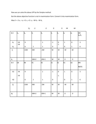
Procedure of Simplex Method
The steps for the computation of an optimum solution are as follows:
Step-1: Check whether the objective function of the given L.P.P is to be maximized or
minimized. If it is to be minimized then we convert it into a problem of maximizing it by using
the result
        Minimum Z = - Maximum(-z)
Step-2: Check whether all right hand side values of the constrains are non-negative. If any one
of values is negative then multiply the           corresponding inequation of the constraints by -1,
so as to get all values are non-negative.
Step-3: Convert all the inequations of the constraints into equations by introducing
slack/surplus variables in the constraints. Put the costs of these variables equal to zero.
Step-4: Obtain an initial basic feasible solution to the problem and put it in the first column of
the simplex table.
Step-5: Compute the net evolutions Δj= Zj – Cj (j=1,2,…..n) by using the         relation Zj – Cj = CB Xj
– Cj .
Examine the sign
        (i)      If all net evolutions are non negative, then the initial basic feasible
        solution is an optimum solution.
        (ii)     If at least one net evolution is negative, proceed on to the next step.
Step-6: If there are more than one negative net evolutions, then choose the most
        negative of them. The corresponding column is called entering            column.
        (i)      If all values in this column are ≤ 0, then there is an unbounded solution to the
given problem.
        (ii)     If at least one value is > 0, then the corresponding variable enters the         basis.


Step-7:Compute the ratio {XB / Entering column} and choose the minimum of     these ratios.
The row which is corresponding to this minimum ratio is called leaving row. The common
element which is in both entering column and leaving row is known as the leading element
or key element        or pivotal element of the table.

Step-8:Convert the key element to unity by dividing its row by the leading      element itself
and all other elements in its column to zeros by using     elementary row transformations.

Step-9:         Go to step-5 and repeat the computational procedure until either an
          optimum solution is obtained or there is an indication of an unbounded solution.
Artificial Variable Technique
– Big M-method

If in a starting simplex table, we don’t have an identity sub matrix (i.e. an obvious starting BFS), then we
introduce artificial variables to have a starting BFS. This is known as artificial variable technique. There is
one method to find the starting BFS and solve the problem i.e., Big M method.

Suppose a constraint equation i does not have a slack variable. i.e. there is no ith unit vector column in
the LHS of the constraint equations. (This happens for example when the ith constraint in the original
LPP is either ≥ or = .) Then we augment the equation with an artificial variable Ai to form the ith unit
vector column. However as the artificial variable is extraneous to the given LPP, we use a feedback
mechanism in which the optimization process automatically attempts to force these variables to zero
level. This is achieved by giving a large penalty to the coefficient of the artificial variable in the objective
function as follows:

Artificial variable objective coefficient

= - M in a maximization problem,

= M in a minimization problem

where M is a very large positive number.

Procedure of Big M-method

The following steps are involved in solving an LPP using the Big M method.

Step-1: Express the problem in the standard form.

Step-2:Add non-negative artificial variables to the left side of each of the equations corresponding to
constraints of the type ≥ or =. However, addition of these artificial variable causes violation of the
corresponding constraints. Therefore, we would like to get rid of these variables and would not allow
them to appear in the final solution. This is achieved by assigning a very large penalty (-M for
maximization and M for minimization) in the objective function.

Step-3:Solve the modified LPP by simplex method, until any one of the three cases may arise.

    1. If no artificial variable appears in the basis and the optimality conditions are satisfied, then the
       current solution is an optimal basic feasible solution.

    2. If at least one artificial variable in the basis at zero level and the optimality condition is satisfied
       then the current solution is an optimal basic feasible solution.

    3. If at least one artificial variable appears in the basis at positive level and the optimality condition
       is satisfied, then the original problem has no feasible solution. The solution satisfies the contains
but does not optimize the objective function, since it contains a very large penalty M and is
        called pseudo optimal solution.

Artificial Variable Technique
– Big M-method

Consider the LPP:

Minimize Z = 2 x1 + x2

Subject to the constraints

       3 x 1 + x2 ≥ 9

         x1 + x2 ≥ 6

          x1, x2 ≥ 0

Putting this in the standard form, the LPP is:

Minimize Z = 2 x1 + x2

Subject to the constraints

       3 x 1 + x 2 – s1        =9

         x1 + x2        – s2 = 6

          x1, x2 ,s1 , s2 ≥ 0

Here s1 , s2 are surplus variables.

Note that we do not have a 2x2 identity sub matrix in the LHS.

Introducing the artificial variables A1, A2 in the above LPP

The modified LPP is as follows:

Minimize Z = 2 x1 + x2 + 0. s1 + 0. s2 + M.A1 + M.A2

Subject to the constraints

       3 x 1 + x 2 – s1        + A1       = 9

         x1 + x2        – s2          + A2 = 6

          x1, x2 , s1 , s2 , A1 , A2 ≥ 0

Note that we now have a 2x2 identity sub matrix in the coefficient matrix of the constraint equations.
Now we can solve the above LPP by the Simplex method.

But the above objective function is not in maximization form. Convert it into maximization form.

Max Z = -2 x1 – x2 + 0. s1 + 0. s2 – M A1 – M A2


                          Cj:        -2             -2        0        0        -M            -M

B.V     CB         XB           X1            X2         S1       S2       A1        A2            MR
                                                                                                   XB/X1


 A1      -M         9                          1          -1       0        1         0              3
         -M                                                       -1
 A2                 6            1             1          0                 0         1              6
 Zj                -15M         -4M           -2M         M        M        -M        -M


Δj                              -4M+2         -2M+1       M        M        0             0
B.V     CB         XB           X1            X2         S1       S2       A1        A2            MR

                                                                                                   XB/X1

 A1      -M         9                          1          -1       0        1         0              3

         -M                                                       -1

 A2                 6            1             1          0                 0         1              6

 Zj                -15M         -4M           -2M         M        M        -M        -M


Δj                              -4M+2         -2M+1       M        M        0             0

Procedure Of Simplex Method

  • 1.
    Procedure of SimplexMethod The steps for the computation of an optimum solution are as follows: Step-1: Check whether the objective function of the given L.P.P is to be maximized or minimized. If it is to be minimized then we convert it into a problem of maximizing it by using the result Minimum Z = - Maximum(-z) Step-2: Check whether all right hand side values of the constrains are non-negative. If any one of values is negative then multiply the corresponding inequation of the constraints by -1, so as to get all values are non-negative. Step-3: Convert all the inequations of the constraints into equations by introducing slack/surplus variables in the constraints. Put the costs of these variables equal to zero. Step-4: Obtain an initial basic feasible solution to the problem and put it in the first column of the simplex table. Step-5: Compute the net evolutions Δj= Zj – Cj (j=1,2,…..n) by using the relation Zj – Cj = CB Xj – Cj . Examine the sign (i) If all net evolutions are non negative, then the initial basic feasible solution is an optimum solution. (ii) If at least one net evolution is negative, proceed on to the next step. Step-6: If there are more than one negative net evolutions, then choose the most negative of them. The corresponding column is called entering column. (i) If all values in this column are ≤ 0, then there is an unbounded solution to the given problem. (ii) If at least one value is > 0, then the corresponding variable enters the basis. Step-7:Compute the ratio {XB / Entering column} and choose the minimum of these ratios. The row which is corresponding to this minimum ratio is called leaving row. The common element which is in both entering column and leaving row is known as the leading element or key element or pivotal element of the table. Step-8:Convert the key element to unity by dividing its row by the leading element itself and all other elements in its column to zeros by using elementary row transformations. Step-9: Go to step-5 and repeat the computational procedure until either an optimum solution is obtained or there is an indication of an unbounded solution.
  • 2.
    Artificial Variable Technique –Big M-method If in a starting simplex table, we don’t have an identity sub matrix (i.e. an obvious starting BFS), then we introduce artificial variables to have a starting BFS. This is known as artificial variable technique. There is one method to find the starting BFS and solve the problem i.e., Big M method. Suppose a constraint equation i does not have a slack variable. i.e. there is no ith unit vector column in the LHS of the constraint equations. (This happens for example when the ith constraint in the original LPP is either ≥ or = .) Then we augment the equation with an artificial variable Ai to form the ith unit vector column. However as the artificial variable is extraneous to the given LPP, we use a feedback mechanism in which the optimization process automatically attempts to force these variables to zero level. This is achieved by giving a large penalty to the coefficient of the artificial variable in the objective function as follows: Artificial variable objective coefficient = - M in a maximization problem, = M in a minimization problem where M is a very large positive number. Procedure of Big M-method The following steps are involved in solving an LPP using the Big M method. Step-1: Express the problem in the standard form. Step-2:Add non-negative artificial variables to the left side of each of the equations corresponding to constraints of the type ≥ or =. However, addition of these artificial variable causes violation of the corresponding constraints. Therefore, we would like to get rid of these variables and would not allow them to appear in the final solution. This is achieved by assigning a very large penalty (-M for maximization and M for minimization) in the objective function. Step-3:Solve the modified LPP by simplex method, until any one of the three cases may arise. 1. If no artificial variable appears in the basis and the optimality conditions are satisfied, then the current solution is an optimal basic feasible solution. 2. If at least one artificial variable in the basis at zero level and the optimality condition is satisfied then the current solution is an optimal basic feasible solution. 3. If at least one artificial variable appears in the basis at positive level and the optimality condition is satisfied, then the original problem has no feasible solution. The solution satisfies the contains
  • 3.
    but does notoptimize the objective function, since it contains a very large penalty M and is called pseudo optimal solution. Artificial Variable Technique – Big M-method Consider the LPP: Minimize Z = 2 x1 + x2 Subject to the constraints 3 x 1 + x2 ≥ 9 x1 + x2 ≥ 6 x1, x2 ≥ 0 Putting this in the standard form, the LPP is: Minimize Z = 2 x1 + x2 Subject to the constraints 3 x 1 + x 2 – s1 =9 x1 + x2 – s2 = 6 x1, x2 ,s1 , s2 ≥ 0 Here s1 , s2 are surplus variables. Note that we do not have a 2x2 identity sub matrix in the LHS. Introducing the artificial variables A1, A2 in the above LPP The modified LPP is as follows: Minimize Z = 2 x1 + x2 + 0. s1 + 0. s2 + M.A1 + M.A2 Subject to the constraints 3 x 1 + x 2 – s1 + A1 = 9 x1 + x2 – s2 + A2 = 6 x1, x2 , s1 , s2 , A1 , A2 ≥ 0 Note that we now have a 2x2 identity sub matrix in the coefficient matrix of the constraint equations.
  • 4.
    Now we cansolve the above LPP by the Simplex method. But the above objective function is not in maximization form. Convert it into maximization form. Max Z = -2 x1 – x2 + 0. s1 + 0. s2 – M A1 – M A2 Cj: -2 -2 0 0 -M -M B.V CB XB X1 X2 S1 S2 A1 A2 MR XB/X1 A1 -M 9 1 -1 0 1 0 3 -M -1 A2 6 1 1 0 0 1 6 Zj -15M -4M -2M M M -M -M Δj -4M+2 -2M+1 M M 0 0 B.V CB XB X1 X2 S1 S2 A1 A2 MR XB/X1 A1 -M 9 1 -1 0 1 0 3 -M -1 A2 6 1 1 0 0 1 6 Zj -15M -4M -2M M M -M -M Δj -4M+2 -2M+1 M M 0 0