Downloaded 904 times
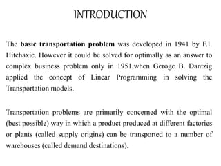
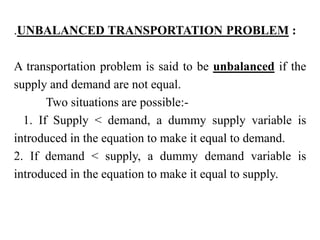
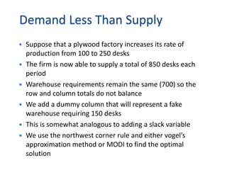
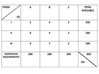
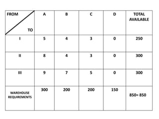
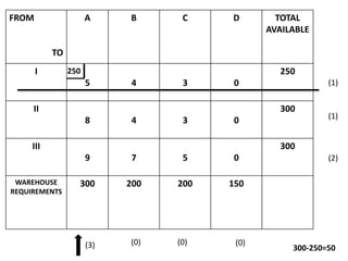
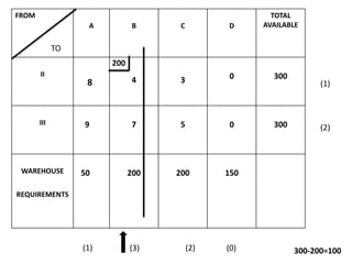
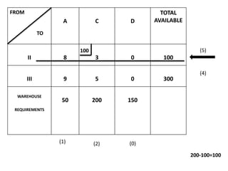
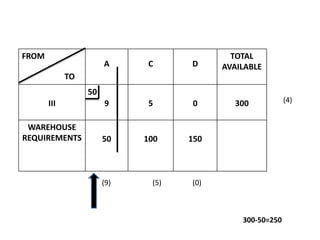
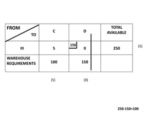
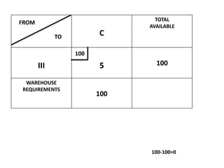
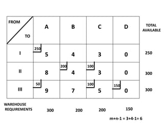
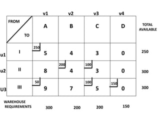
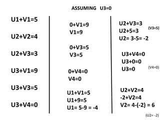
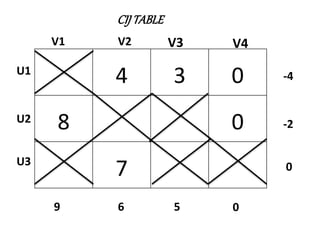
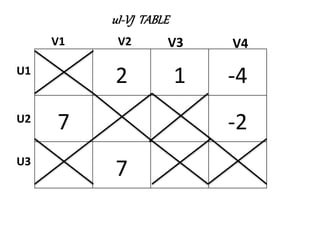
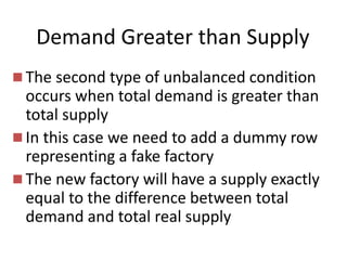
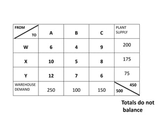
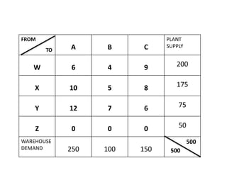
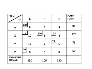
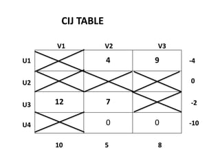
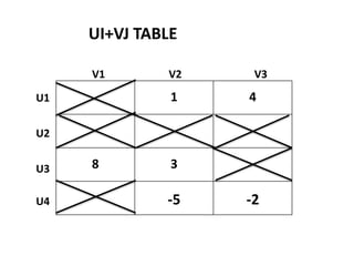
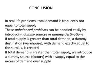


The document discusses transportation problems and their optimization using linear programming. It begins by explaining that transportation problems aim to optimally transport goods from supply origins to demand destinations at minimum cost while satisfying supply and demand constraints. The document then discusses how balanced transportation problems have equal total supply and demand, while unbalanced problems introduce dummy variables to balance totals. It provides examples of unbalanced problems where supply exceeds demand and vice versa, and how dummy columns/rows are added to balance the problems and find optimal solutions.