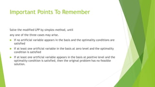
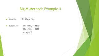
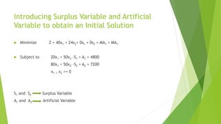
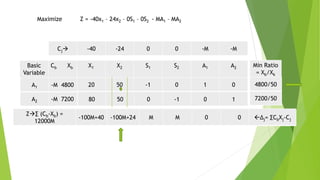
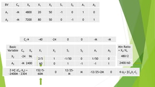
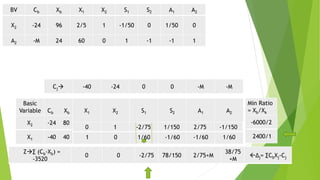
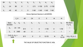
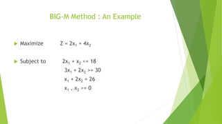
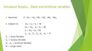
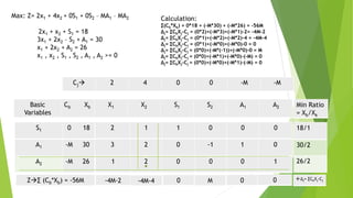
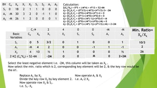
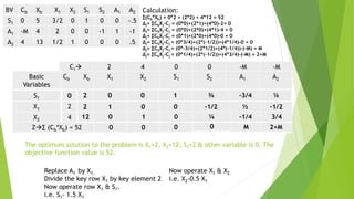
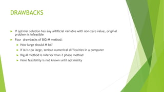
The document describes the Big-M method, a variation of the simplex method for solving linear programming problems with "greater-than" or "equal-to" constraints. It involves adding artificial variables to obtain an initial feasible solution, using a large value M for each artificial variable. The transformed problem is then solved via simplex method to eliminate artificial variables. Examples are provided to illustrate the step-by-step process. Potential drawbacks discussed are how large M should be and not knowing feasibility until optimality is reached.

1. BIG-M METHOD
A VARIANT OF SIMPLEX METHOD
PRESENTED BY:
NISHIDH VILAS LAD-2013176
NITESH BERIWAL-2013177
NITESH SINGH PATEL-2013178
NITIN BORATWAR-2013179
NITIN KUMAR SHUKLA-2013180
NOOPUR MANDHYAN-2013181

2. INTRODUCTION
WHAT IS BIG-M METHOD?
 The Big M method is a method of solving linear programming problems.
 It is a variation of the simplex method designed for solving problems typically
encompassing "greater-than" constraints as well as "less-than" constraints -
where the zero vector is not a feasible solution.
 The "Big M" refers to a large number associated with the artificial variables,
represented by the letter M.

3. Steps In The Big-M Method
 Add artificial variables in the model to obtain a feasible solution.
 Added only to the ‘>’ type or the ‘=‘ constraints
 A value M is assigned to each artificial variable
 The transformed problem is then solved using simplex eliminating the
artificial variables

4. Important Points To Remember
Solve the modified LPP by simplex method, until
any one of the three cases may arise.
 If no artificial variable appears in the basis and the optimality conditions are
satisfied
 If at least one artificial variable in the basis at zero level and the optimality
condition is satisfied
 If at least one artificial variable appears in the basis at positive level and the
optimality condition is satisfied, then the original problem has no feasible
solution.

5. Big M Method: Example 1
 Minimize Z = 40x1 + 24x2
 Subject to 20x1 + 50x2 >= 4800
80x1 + 50x2 >= 7200
x1 , x2 >= 0

6. Introducing Surplus Variable and Artificial
Variable to obtain an Initial Solution
 Minimize Z = 40x1 + 24x2+ 0s1 + 0s2 + MA1 + MA1
 Subject to 20x1 + 50x2 –S1 + A1 = 4800
80x1 + 50x2 –S2 + A2 = 7200
x1 , x2 >= 0
S1 and S2 Surplus Variable
A1 and A2 Artificial Variable

7. Basic
Variable
s
Cb Xb X1 X2 S1 S2 A1 A2
Cj -40 -24 0 0 -M -M
A1 -M 4800
A2 -M 7200
20 50 -1 0 1 0
80 50 0 -1 0 1
Z∑ (Cb-Xb) =
12000M
-100M+40 -100M+24 M M 0 0 ∆j= ∑CbXj-Cj
Min Ratio
= Xb/Xk
4800/50
7200/50
Maximize Z = -40x1 – 24x2 – 0S1 – 0S2 - MA1 – MA2

8. Basic
Variable
s
Cb Xb X1 X2 S1 S2 A1 A2
Cj -40 -24 0 0 -M -M
X2 -24 96
A2 -M 2400 60 0 1 -1 -1 1
Z∑ (Cb-Xb) =
-2400M - 2304
152/5-
60M
0
12/25-
M
M -12/25+2M 0 ∆j= ∑CbXj-Cj
Min Ratio
= Xb/Xk
480/2
2400/60
2/5 1 -1/50 0 1/50 0
BV Cb Xb X1 X2 S1 S2 A1 A2
A1 -M 4800 20 50 -1 0 1 0
A2 -M 7200 80 50 0 -1 0 1

9. Basic
Variable
s
Cb Xb X1 X2 S1 S2 A1 A2
Cj -40 -24 0 0 -M -M
X2 -24 80
X1 -40 40 1 0 1/60 -1/60 -1/60 1/60
Z∑ (Cb-Xb) =
-3520
0 0 -2/75 78/150 2/75+M
38/75
+M
∆j= ∑CbXj-Cj
Min Ratio
= Xb/Xk
-6000/2
2400/1
0 1 -2/75 1/150 2/75 -1/150
BV Cb Xb X1 X2 S1 S2 A1 A2
X2 -24 96 2/5 1 -1/50 0 1/50 0
A2 -M 24 60 0 1 -1 -1 1

10. Basic
Variable
s
Cb Xb X1 X2 S1 S2 A1 A2
Cj -40 -24 0 0 -M -M
X2 -24 144
S1 0 2400 60 0 1 -1 -1 1
Z∑ (Cb-Xb) =
3456
8/5 0 0 12/25 M
M-
12/25
∆j= ∑CbXj-Cj
Min Ratio
= Xb/Xk
_
_
8/5 1 0 -1/50 0 1/50
THE VALUE OF OBJECTIVE FUNCTION IS 3456
BV Cb Xb X1 X2 S1 S2 A1 A2
X2 -24 80 0 1 -2/5 1/150 2/75 -1/150
X1 -40 40 1 0 1/60 -1/60 -1/60 1/60
Hence Optimal Solution is ACHIEVED.

11. BIG-M Method : An Example
 Maximize Z = 2x1 + 4x2
 Subject to 2x1 + x2 <= 18
3x1 + 2x2 >= 30
x1 + 2x2 = 26
x1 , x2 >= 0

12. Introduce Surplus , Slack and Artificial variables
 Maximize Z = 2x1 + 4x2 + 0S1 + 0S2 – MA1 – MA2
 Subject to 2x1 + x2 + S1 = 18
3x1 + 2x2 – S2 + A1 = 30
x1 + 2x2 + A2 = 26
x1 , x2 , S1 , S2 , A1 , A2 >= 0
S1 -> Slack Variable
S2 -> Surplus Variable
A1 , A2 -> Artificial Variable
M -> Large value

13. Max: Z= 2x1 + 4x2 + 0S1 + 0S2 – MA1 – MA2
2x1 + x2 + S1 = 18
3x1 + 2x2 – S2 + A1 = 30
x1 + 2x2 + A2 = 26
x1 , x2 , S1 , S2 , A1 , A2 >= 0
Z∑ (Cb*Xb) = -56M
Basic
Variables
Cb Xb X1 X2 S1 S2 A1 A2
S1 0 18
A1 -M 30
A2 -M 26
2 1 1 0 0 0
3 2 0 -1 1 0
1 2 0 0 0 1
Min Ratio
= Xb/Xk
18/1
30/2
26/2
Cj 2 4 0 0 -M -M
Calculation:
∑(Cb*Xb) = 0*18 + (-M*30) + (-M*26) = -56M
∆j= ∑CbXj-Cj = (0*2)+(-M*3)+(-M*1)-2= -4M-2
∆j= ∑CbXj-Cj = (0*1)+(-M*2)+(-M*2)-4 = -4M-4
∆j= ∑CbXj-Cj = (0*1)+(-M*0)+(-M*0)-0 = 0
∆j= ∑CbXj-Cj = (0*0)+(-M*(-1))+(-M*0)-0 = M
∆j= ∑CbXj-Cj = (0*0)+(-M*1)+(-M*0)-(-M) = 0
∆j= ∑CbXj-Cj = (0*0)+(-M*0)+(-M*1)-(-M) = 0
∆j= ∑CbXj-Cj0M0-4M-4-4M-2 0

14. BV Cb Xb X1 X2 S1 S2 A1 A2
S1 0 18 2 1 1 0 0 0
A1 -M 30 3 2 0 -1 1 0
A2 -M 26 1 2 0 0 0 1
Cj 2 4 0 0 -M -M
Basic
Variables
Cb Xb X1 X2 S1 S2 A1 A2
S1
A1
X2
0
-M
4
Replace A2 by X2.
Divide the key row X2 by key element 2.
Now operate row X2 & S1.
i.e. S1- X2
13 ½ 1 0 0 0 ½
5 3/2 0 1 0 0 1
Now operate A1 & X2
i.e. A1-2 X2
4 2 0 0 -1 1 -1
Z∑ (Cb*Xb) = 52-4M
Calculation:
∑(Cb*Xb) = 0*5 + (-M*4) + 4*13 = 52-4M
∆j= ∑CbXj-Cj = (0*3/2)+(-M*2)+(4*1/2)-2= -2M
∆j= ∑CbXj-Cj = (0*0)+(-M*0)+(4*1)-4 = 0
∆j= ∑CbXj-Cj = (0*1)+(-M*0)+(4*0)-0 = 0
∆j= ∑CbXj-Cj = (0*0)+(-M*(-1))+(4*0)-0 = M
∆j= ∑CbXj-Cj = (0*0)+(-M*1)+(4*0)-(-M) = 0
∆j= ∑CbXj-Cj = (0*1)+(-M*(-1))+(4*1/2)-(-M) = 2+2M
-2M 0 0 M 0 2+2M
Select the least negative element i.e. -2M, this column will be taken as Xk .
Now select the min. ratio which is 2, corresponding key element will be 2, & the key row would be
the A1.
Min. Ratio=
Xb/Xk
10/3
2
26

15. BV Cb Xb X1 X2 S1 S2 A1 A2
S1 0 5 3/2 0 1 0 0 -.5
A1 -M 4 2 0 0 -1 1 -1
A2 4 13 1/2 1 0 0 0 .5
Cj 2 4 0 0 -M -M
Basic
Variables
Cb Xb X1 X2 S1 S2 A1 A2
S1
X1
X2
0
2
4
Replace A1 by X1.
Divide the key row X1 by key element 2
Now operate row X1 & S1.
i.e. S1- 1.5 X1
2 0 0 1 ¾ -3/4 ¼
Now operate X1 & X2
i.e. X2-0.5 X1
Z∑ (Cb*Xb) = 52
Calculation:
∑(Cb*Xb) = 0*2 + (2*2) + 4*12 = 52
∆j= ∑CbXj-Cj = (0*0)+(2*1)+(4*0)-2= 0
∆j= ∑CbXj-Cj = (0*0)+(2*0)+(4*1)-4 = 0
∆j= ∑CbXj-Cj = (0*1)+(2*0)+(4*0)-0 = 0
∆j= ∑CbXj-Cj = (0*3/4)+(2*(-1/2))+(4*1/4)-0 = 0
∆j= ∑CbXj-Cj = (0*-3/4)+(2*1/2)+(4*(-1/4))-(-M) = M
∆j= ∑CbXj-Cj = (0*1/4)+(2*(-1/2))+(4*3/4)-(-M) = 2+M
0 0 0 0 M 2+M
2 1 0 0 -1/2 ½ -1/2
12 0 1 0 ¼ -1/4 3/4
The optimum solution to the problem is X1=2, X2=12, S1=2 & other variable is 0. The
objective function value is 52.

16. DRAWBACKS
 If optimal solution has any artificial variable with non-zero value, original
problem is infeasible
 Four drawbacks of BIG-M method:
 How large should M be?
 If M is too large, serious numerical difficulties in a computer
 Big-M method is inferior than 2 phase method
 Here feasibility is not known until optimality