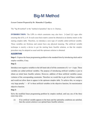
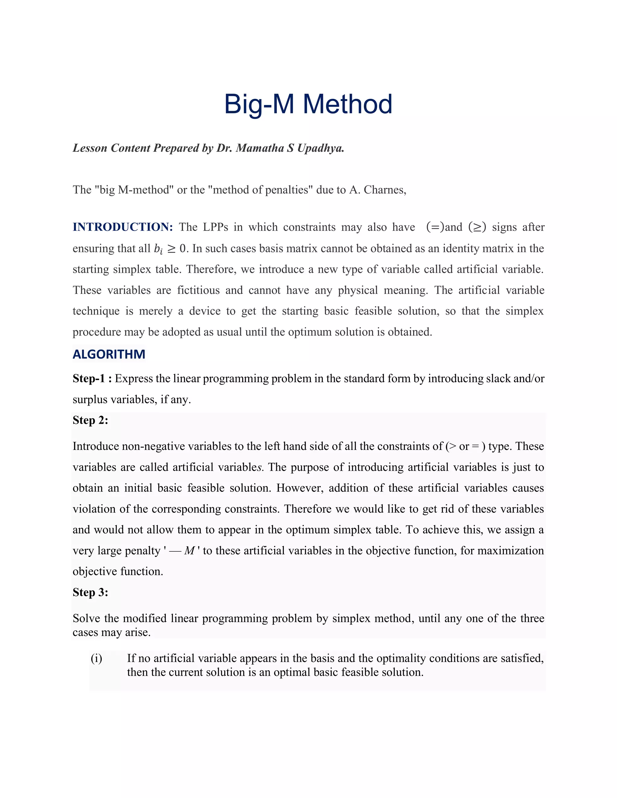
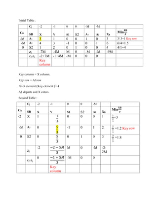
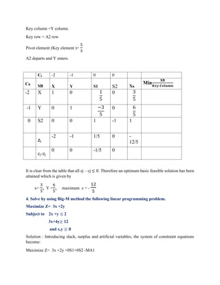
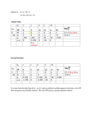
Big-M Method
Lesson Content Prepared by Dr. Mamatha S Upadhya.
The "big M-method" or the "method of penalties" due to A. Charnes,
INTRODUCTION: The LPPs in which constraints may also have (=)and (≥) signs after
ensuring that all 𝑏𝑖 ≥ 0. In such cases basis matrix cannot be obtained as an identity matrix in the
starting simplex table. Therefore, we introduce a new type of variable called artificial variable.
These variables are fictitious and cannot have any physical meaning. The artificial variable
technique is merely a device to get the starting basic feasible solution, so that the simplex
procedure may be adopted as usual until the optimum solution is obtained.
ALGORITHM
Step-1 : Express the linear programming problem in the standard form by introducing slack and/or
surplus variables, if any.
Step 2:
Introduce non-negative variables to the left hand side of all the constraints of (> or = ) type. These
variables are called artificial variables. The purpose of introducing artificial variables is just to
obtain an initial basic feasible solution. However, addition of these artificial variables causes
violation of the corresponding constraints. Therefore we would like to get rid of these variables
and would not allow them to appear in the optimum simplex table. To achieve this, we assign a
very large penalty ' — M ' to these artificial variables in the objective function, for maximization
objective function.
Step 3:
Solve the modified linear programming problem by simplex method, until any one of the three
cases may arise.
(i) If no artificial variable appears in the basis and the optimality conditions are satisfied,
then the current solution is an optimal basic feasible solution.
(ii) If at least one artificial variable is there in the basis at zero level and the optimality
condition is satisfied, then the current solution is an optimal basic feasible
solution(though degenerated)
(iii) If at least one artificial variable appears in the basis at positive level and the optimality
condition is satisfied, then the original problem has no feasible solution.
Note: while applying simplex method, whenever an artificial variable happens to leave the basis,
we drop that artificial variable and omit all the entries corresponding to its column from the
simplex table.
Illustration:
1. Solve by using Big-M method the following linear programming problem.
Maximize z = x1 + 5x2
Subject to
3x1 +4x2 ≤ 6
x1 + 3x2 ≥ 2
x1, x2 ≥ 0
Solution:
Converting inequalities to equalities
By introducing surplus variables, slack variables and artificial variables, the standard form of LPP
becomes
Maximize Z= x1 + 5x2 + 0S1 + 0S2 – MA1
Subject to
3x1 + 4x2 + S1 = 6
x1 + 3x2 – S2+ A1 = 2
x1 ≥ 0, x2 ≥ 0, S1 ≥ 0, S2 ≥ 0, A1≥ 0
where,
S1 is a slack variable
S2 is a surplus variable
A1 is an artificial variable.
Initial Table
Cj 1 5 0 0 –M
CB
Basic
variables
SB
x1 x2 S1 S2 A1
Solution
values
b (= XB)
Ratio Min
(
𝐗𝐁
𝑲𝒆𝒚 𝑪𝒐𝒍𝒖𝒎𝒏
)
0 S1 3 4 1 0 0 6
𝟔
𝟒
=1.5
–M A1 1 3 0 –1 1 2
𝟐
𝟑
=0.66
zj -M -3M 0 M -M
cj-zj 1+M 5+3M 0 -M 0
Key
Column
As M is a large positive number, Max (cj − zj ) is 5+3M , hence , x2 becomes a basic variable
in the next iteration.
Key column = x2 column.
Minimum (6/4, 2/3) = 2/3
Key row = A1 row
Pivot element (Key element )= 3.
A1 departs and x2 enters.
Iteration 2:
Note: The iteration just completed, artificial variable A1 was eliminated from the basis. The new
solution is shown in the following table.
Cj 1 5 0 0
CB
Basic
variables
SB
x1 x2 S1 S2
Solution
values
b (= XB)
Ratio Min
(
𝐗𝐁
𝑲𝒆𝒚 𝑪𝒐𝒍𝒖𝒎𝒏
)
0 S1
𝟓
𝟑
0 1
4
3
10
3
10/4 =2.5
5 x2
𝟏
𝟑
1 0 –
1
3
𝟐
𝟑
-Ve
zj
𝟓
𝟑
5 0 –
5
3
10
3
cj-zj -
𝟐
𝟑
0 0
𝟓
𝟑
Key
Column
Iteration 3:
Cj 1 5 0 0
CB
Basic
variables
SB
x1 x2 S1 S2
Solution
values
b (= XB)
Ratio Min
(
𝐗𝐁
𝑲𝒆𝒚 𝑪𝒐𝒍𝒖𝒎𝒏
)
0 S2
𝟓
𝟒
0
𝟑
𝟒
1
𝟓
𝟐
5 x2
𝟑
𝟒
1
𝟏
𝟒
0
𝟑
𝟐
zj
𝟏𝟓
𝟒
5
𝟓
𝟒
0
𝟏𝟓
𝟐
cj-zj −
𝟏𝟏
𝟒
0 -
𝟓
𝟒
0
Result: Since, all cj-zj ≤ 0, The optimal solution is x1 = 0, x2 = 3/2 and Max z =15/2
2. Use penalty (or Big 'M') method to
Minimize z = 4xi + 3x2
subject to the constraints:
2x1+ x2 ≥ 10,
-3x1, + 2x2 ≤ 6
x1 + x2 ≥ 6,
x1 ≥ 0 and x2 ≥ 0.
Solution. Introducing surplus (negative slack) variables x3 ≥ 0, x5 ≥ 0 and slack variable x4 ≥
0 in the constraint inequations, We introduce two new variables A1 ≥ 0 and A2 ≥ 0 in the first and
third equations respectively. These extraneous variables, commonly termed as artificial variables,
play the same role as that of slack variables in providing a starting basic feasible solution.
Since the objective function is minimization, we convert it into maximization using,
Min Z = -Max (-Z)= - Max Z*
The problem becomes
Maximize z* = - 4x1 - 3x2 + 0.S1 + 0.S2 + 0.S3 – MA1- MA2
Subject to the constraints:
2x1 + x2 - S1 + A1= 10
- 3x1 + 2x2 + S2 = 6
xl + x2 – S3+ A2 = 6,
xj ≥ 0 (j = 1,2, 3, 4, 5)
Initial Table:
Cj -4 -3 0 0 0 -M -M
CB
SB x1 x2 S1 S2 S3 A1 A2 XB
Min
𝐗𝐁
𝑿𝟏
-M A1 2 1 -1 0 0 1 0 10 10/2=5 Key row
0 S2 -3 2 0 1 0 0 0 6 -ve
_-M A2 1 1 0 0 -1 0 1 6 6
zj
-3M -2M M 0 M -M -M -
16M
cj-zj -4+3M -3+2M -M 0 -M 0 0
Key
column
Key column = x1 column.
Key row = A1 row
Pivot element (Key element )= 2.
A1 departs and x1 enters.
Second Table :
Cj -4 -3 0 0 0 -M
CB
SB x1 x2 S1 S2 S3 A2 XB
Min
𝐗𝐁
𝑿𝟐
-4 x1 1 1
2
-
1
2
0 0 0 5 5/2=2.5
0 S2 0 7
2
-
3
2
1 0 0 21 21/6
-M A2 0 1
2
1
2
0 -1 0 1 ½=0.5 Key row
zj
-4 −4 − 𝑀
2
4 − 𝑀
2
0 M 0
cj-zj
0 −2 + 𝑀
2
−4 + 𝑀
2
0 -M -M
Key
column
Key column = x2 column.
Key row = A2 row
Pivot element (Key element )= 1/2
A2 departs and x2 enters.
Cj -4 -3 0 0 0
CB
SB x1 x2 S1 S2 S3 XB
Min
𝐗𝐁
𝑿𝟐
-4 x1 1 0 -1 0 1 4
0 S2 0 0 -5 1 7 14
-3 x2 0 1 1 0 -2 2
zj -4 -3 1 0 2 -22
cj-zj 0 0 -1 0 -2
It is clear from the table that all zj – cj ≤ 0. Therefore an optimum basic feasible solution has been
attained which is given by
x1= 4, x2 = 2, maximum z = -22.
Therefore Min Z = - Max Z* = 22 , at x1= 4, x2 = 2
3. Solve by using Big-M method the following linear programming problem.
Maximize Z= -2 x-y
Subject to 3x +y = 3
4x+3y≥ 6
x+2y≤ 4
and x,y ≥ 𝟎
Introducing slack, surplus and artificial variables, the system of constraint equations become:
Maximize Z= -2 x-y +0S1+0S2 -MA1-MA2
Subject to 3x +y +A1= 3
4x+3y−𝑆1 +A2= 6
x+2y+ 𝑆2 = 4
Initial Table :
Cj -2 -1 0 0 -M -M
CB
SB X Y S1 S2 A1 A2 XB
Min
𝐗𝐁
𝑿
-M A1 3 1 0 0 1 0 3 3/ 3=1 Key row
-M A2 4 3 -1 0 0 1 6 6/4=1.5
0 S2 1 2 0 1 0 0 4 4/1=4
zj -7M -4M M 0 -M -M -9M
cj-zj -2+7M -1+4M -M 0 0 0
Key
column
Key column = X column.
Key row = A1row
Pivot element (Key element )= 4
A1 departs and X enters.
Second Table :
Cj -2 -1 0 0 -M
CB
SB X Y S1 S2 A2 XB
Min
𝐗𝐁
𝒚
-2 X 1 1
3
0 0 0 1 1
1
3
=3
-M A2 0 5
3
-1 0 1 2 2
5
3
=1.2 Key row
0 S2 0 5
3
0 1 0 3 3
5
3
=1.8
zj
-2 −2 − 5𝑀
3
M 0 -M -2-
2M
cj-zj
0 −1 + 5𝑀
3
-M 0 0
Key
column
Key column =Y column.
Key row = A2 row
Pivot element (Key element )=
5
3
A2 departs and Y enters.
Cj -2 -1 0 0
CB
SB X Y S1 S2 XB
Min
𝐗𝐁
𝑲𝒆𝒚 𝑪𝒐𝒍𝒖𝒎𝒏
-2 X 1 0 1
5
0 3
5
-1 Y 0 1 −3
5
0 6
5
0 S2 0 0 1 -1 1
zj
-2 -1 1/5 0 -
12/5
cj-zj
0 0 -1/5 0
It is clear from the table that all zj – cj ≤ 0. Therefore an optimum basic feasible solution has been
attained which is given by
x=
3
5
, Y =
6
5
, maximum z = -
12
5
4. Solve by using Big-M method the following linear programming problem.
Maximize Z= 3x +2y
Subject to 2x +y ≤ 2
3x+4y≥ 12
and x,y ≥ 𝟎
Solution : Introducing slack, surplus and artificial variables, the system of constraint equations
become:
Maximize Z= 3x +2y +0S1+0S2 -MA1
Subject to 2x +y +S1= 2
3x+4y−𝑆2+A1= 12
Initial Table
Cj 3 2 0 0 -M
CB
SB X Y S1 S2 A1 XB
Min
𝐗𝐁
𝒀
0 S1 2 1 1 0 0 2 2/1=2 Key Row
-M A1 3 4 0 -1 1 12 12/4=3
zj -3M -4M 0 M -M -12M
cj-zj 0 2+4M 0 -M 0
Key
column
Second Iteration
Cj 3 2 0 0 -M
CB
SB X Y S1 S2 A1 XB
Min
𝐗𝐁
𝒀
2 Y 2 1 1 0 0 2 2/1=2 Key Row
-M A1 -5 0 -4 -1 1 4 12/4=3
zj 4+5M 2 2+4M M -M 4-4M
cj-zj -1-5M 0 -2-4M -M 0
It is clear from the table that all zj – cj ≤ 0 and an artificial variable appears in the basis , the LPP
does not posses any feasible solution . But the LPP posses a pseudo optimal solution.

Big m method

  • 1.
    Big-M Method Lesson ContentPrepared by Dr. Mamatha S Upadhya. The "big M-method" or the "method of penalties" due to A. Charnes, INTRODUCTION: The LPPs in which constraints may also have (=)and (≥) signs after ensuring that all 𝑏𝑖 ≥ 0. In such cases basis matrix cannot be obtained as an identity matrix in the starting simplex table. Therefore, we introduce a new type of variable called artificial variable. These variables are fictitious and cannot have any physical meaning. The artificial variable technique is merely a device to get the starting basic feasible solution, so that the simplex procedure may be adopted as usual until the optimum solution is obtained. ALGORITHM Step-1 : Express the linear programming problem in the standard form by introducing slack and/or surplus variables, if any. Step 2: Introduce non-negative variables to the left hand side of all the constraints of (> or = ) type. These variables are called artificial variables. The purpose of introducing artificial variables is just to obtain an initial basic feasible solution. However, addition of these artificial variables causes violation of the corresponding constraints. Therefore we would like to get rid of these variables and would not allow them to appear in the optimum simplex table. To achieve this, we assign a very large penalty ' — M ' to these artificial variables in the objective function, for maximization objective function. Step 3: Solve the modified linear programming problem by simplex method, until any one of the three cases may arise. (i) If no artificial variable appears in the basis and the optimality conditions are satisfied, then the current solution is an optimal basic feasible solution.
  • 2.
    (ii) If atleast one artificial variable is there in the basis at zero level and the optimality condition is satisfied, then the current solution is an optimal basic feasible solution(though degenerated) (iii) If at least one artificial variable appears in the basis at positive level and the optimality condition is satisfied, then the original problem has no feasible solution. Note: while applying simplex method, whenever an artificial variable happens to leave the basis, we drop that artificial variable and omit all the entries corresponding to its column from the simplex table. Illustration: 1. Solve by using Big-M method the following linear programming problem. Maximize z = x1 + 5x2 Subject to 3x1 +4x2 ≤ 6 x1 + 3x2 ≥ 2 x1, x2 ≥ 0 Solution: Converting inequalities to equalities By introducing surplus variables, slack variables and artificial variables, the standard form of LPP becomes Maximize Z= x1 + 5x2 + 0S1 + 0S2 – MA1 Subject to 3x1 + 4x2 + S1 = 6 x1 + 3x2 – S2+ A1 = 2 x1 ≥ 0, x2 ≥ 0, S1 ≥ 0, S2 ≥ 0, A1≥ 0 where, S1 is a slack variable S2 is a surplus variable A1 is an artificial variable.
  • 3.
    Initial Table Cj 15 0 0 –M CB Basic variables SB x1 x2 S1 S2 A1 Solution values b (= XB) Ratio Min ( 𝐗𝐁 𝑲𝒆𝒚 𝑪𝒐𝒍𝒖𝒎𝒏 ) 0 S1 3 4 1 0 0 6 𝟔 𝟒 =1.5 –M A1 1 3 0 –1 1 2 𝟐 𝟑 =0.66 zj -M -3M 0 M -M cj-zj 1+M 5+3M 0 -M 0 Key Column As M is a large positive number, Max (cj − zj ) is 5+3M , hence , x2 becomes a basic variable in the next iteration. Key column = x2 column. Minimum (6/4, 2/3) = 2/3 Key row = A1 row Pivot element (Key element )= 3. A1 departs and x2 enters. Iteration 2: Note: The iteration just completed, artificial variable A1 was eliminated from the basis. The new solution is shown in the following table.
  • 4.
    Cj 1 50 0 CB Basic variables SB x1 x2 S1 S2 Solution values b (= XB) Ratio Min ( 𝐗𝐁 𝑲𝒆𝒚 𝑪𝒐𝒍𝒖𝒎𝒏 ) 0 S1 𝟓 𝟑 0 1 4 3 10 3 10/4 =2.5 5 x2 𝟏 𝟑 1 0 – 1 3 𝟐 𝟑 -Ve zj 𝟓 𝟑 5 0 – 5 3 10 3 cj-zj - 𝟐 𝟑 0 0 𝟓 𝟑 Key Column Iteration 3: Cj 1 5 0 0 CB Basic variables SB x1 x2 S1 S2 Solution values b (= XB) Ratio Min ( 𝐗𝐁 𝑲𝒆𝒚 𝑪𝒐𝒍𝒖𝒎𝒏 ) 0 S2 𝟓 𝟒 0 𝟑 𝟒 1 𝟓 𝟐 5 x2 𝟑 𝟒 1 𝟏 𝟒 0 𝟑 𝟐 zj 𝟏𝟓 𝟒 5 𝟓 𝟒 0 𝟏𝟓 𝟐 cj-zj − 𝟏𝟏 𝟒 0 - 𝟓 𝟒 0 Result: Since, all cj-zj ≤ 0, The optimal solution is x1 = 0, x2 = 3/2 and Max z =15/2
  • 5.
    2. Use penalty(or Big 'M') method to Minimize z = 4xi + 3x2 subject to the constraints: 2x1+ x2 ≥ 10, -3x1, + 2x2 ≤ 6 x1 + x2 ≥ 6, x1 ≥ 0 and x2 ≥ 0. Solution. Introducing surplus (negative slack) variables x3 ≥ 0, x5 ≥ 0 and slack variable x4 ≥ 0 in the constraint inequations, We introduce two new variables A1 ≥ 0 and A2 ≥ 0 in the first and third equations respectively. These extraneous variables, commonly termed as artificial variables, play the same role as that of slack variables in providing a starting basic feasible solution. Since the objective function is minimization, we convert it into maximization using, Min Z = -Max (-Z)= - Max Z* The problem becomes Maximize z* = - 4x1 - 3x2 + 0.S1 + 0.S2 + 0.S3 – MA1- MA2 Subject to the constraints: 2x1 + x2 - S1 + A1= 10 - 3x1 + 2x2 + S2 = 6 xl + x2 – S3+ A2 = 6, xj ≥ 0 (j = 1,2, 3, 4, 5)
  • 6.
    Initial Table: Cj -4-3 0 0 0 -M -M CB SB x1 x2 S1 S2 S3 A1 A2 XB Min 𝐗𝐁 𝑿𝟏 -M A1 2 1 -1 0 0 1 0 10 10/2=5 Key row 0 S2 -3 2 0 1 0 0 0 6 -ve _-M A2 1 1 0 0 -1 0 1 6 6 zj -3M -2M M 0 M -M -M - 16M cj-zj -4+3M -3+2M -M 0 -M 0 0 Key column Key column = x1 column. Key row = A1 row Pivot element (Key element )= 2. A1 departs and x1 enters. Second Table : Cj -4 -3 0 0 0 -M CB SB x1 x2 S1 S2 S3 A2 XB Min 𝐗𝐁 𝑿𝟐 -4 x1 1 1 2 - 1 2 0 0 0 5 5/2=2.5 0 S2 0 7 2 - 3 2 1 0 0 21 21/6 -M A2 0 1 2 1 2 0 -1 0 1 ½=0.5 Key row zj -4 −4 − 𝑀 2 4 − 𝑀 2 0 M 0 cj-zj 0 −2 + 𝑀 2 −4 + 𝑀 2 0 -M -M Key column
  • 7.
    Key column =x2 column. Key row = A2 row Pivot element (Key element )= 1/2 A2 departs and x2 enters. Cj -4 -3 0 0 0 CB SB x1 x2 S1 S2 S3 XB Min 𝐗𝐁 𝑿𝟐 -4 x1 1 0 -1 0 1 4 0 S2 0 0 -5 1 7 14 -3 x2 0 1 1 0 -2 2 zj -4 -3 1 0 2 -22 cj-zj 0 0 -1 0 -2 It is clear from the table that all zj – cj ≤ 0. Therefore an optimum basic feasible solution has been attained which is given by x1= 4, x2 = 2, maximum z = -22. Therefore Min Z = - Max Z* = 22 , at x1= 4, x2 = 2 3. Solve by using Big-M method the following linear programming problem. Maximize Z= -2 x-y Subject to 3x +y = 3 4x+3y≥ 6 x+2y≤ 4 and x,y ≥ 𝟎 Introducing slack, surplus and artificial variables, the system of constraint equations become: Maximize Z= -2 x-y +0S1+0S2 -MA1-MA2 Subject to 3x +y +A1= 3 4x+3y−𝑆1 +A2= 6 x+2y+ 𝑆2 = 4
  • 8.
    Initial Table : Cj-2 -1 0 0 -M -M CB SB X Y S1 S2 A1 A2 XB Min 𝐗𝐁 𝑿 -M A1 3 1 0 0 1 0 3 3/ 3=1 Key row -M A2 4 3 -1 0 0 1 6 6/4=1.5 0 S2 1 2 0 1 0 0 4 4/1=4 zj -7M -4M M 0 -M -M -9M cj-zj -2+7M -1+4M -M 0 0 0 Key column Key column = X column. Key row = A1row Pivot element (Key element )= 4 A1 departs and X enters. Second Table : Cj -2 -1 0 0 -M CB SB X Y S1 S2 A2 XB Min 𝐗𝐁 𝒚 -2 X 1 1 3 0 0 0 1 1 1 3 =3 -M A2 0 5 3 -1 0 1 2 2 5 3 =1.2 Key row 0 S2 0 5 3 0 1 0 3 3 5 3 =1.8 zj -2 −2 − 5𝑀 3 M 0 -M -2- 2M cj-zj 0 −1 + 5𝑀 3 -M 0 0 Key column
  • 9.
    Key column =Ycolumn. Key row = A2 row Pivot element (Key element )= 5 3 A2 departs and Y enters. Cj -2 -1 0 0 CB SB X Y S1 S2 XB Min 𝐗𝐁 𝑲𝒆𝒚 𝑪𝒐𝒍𝒖𝒎𝒏 -2 X 1 0 1 5 0 3 5 -1 Y 0 1 −3 5 0 6 5 0 S2 0 0 1 -1 1 zj -2 -1 1/5 0 - 12/5 cj-zj 0 0 -1/5 0 It is clear from the table that all zj – cj ≤ 0. Therefore an optimum basic feasible solution has been attained which is given by x= 3 5 , Y = 6 5 , maximum z = - 12 5 4. Solve by using Big-M method the following linear programming problem. Maximize Z= 3x +2y Subject to 2x +y ≤ 2 3x+4y≥ 12 and x,y ≥ 𝟎 Solution : Introducing slack, surplus and artificial variables, the system of constraint equations become: Maximize Z= 3x +2y +0S1+0S2 -MA1
  • 10.
    Subject to 2x+y +S1= 2 3x+4y−𝑆2+A1= 12 Initial Table Cj 3 2 0 0 -M CB SB X Y S1 S2 A1 XB Min 𝐗𝐁 𝒀 0 S1 2 1 1 0 0 2 2/1=2 Key Row -M A1 3 4 0 -1 1 12 12/4=3 zj -3M -4M 0 M -M -12M cj-zj 0 2+4M 0 -M 0 Key column Second Iteration Cj 3 2 0 0 -M CB SB X Y S1 S2 A1 XB Min 𝐗𝐁 𝒀 2 Y 2 1 1 0 0 2 2/1=2 Key Row -M A1 -5 0 -4 -1 1 4 12/4=3 zj 4+5M 2 2+4M M -M 4-4M cj-zj -1-5M 0 -2-4M -M 0 It is clear from the table that all zj – cj ≤ 0 and an artificial variable appears in the basis , the LPP does not posses any feasible solution . But the LPP posses a pseudo optimal solution.