The document discusses the transportation problem in operations research and linear programming. It can be summarized as:
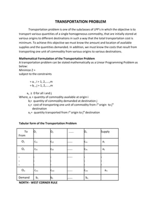
1) The transportation problem aims to transport goods from multiple origins to multiple destinations in a way that minimizes total transportation costs, given supply and demand constraints.
2) It can be formulated as a linear programming problem to find the optimal amounts transported between each origin-destination pair to minimize costs.
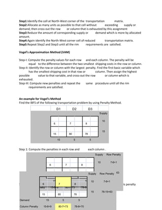
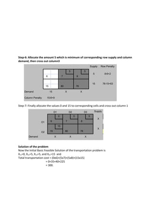
3) Solution methods like the Northwest Corner Rule and Vogel's Approximation Method are presented to find initial basic feasible solutions for the transportation problem.