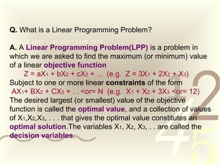
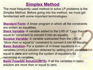
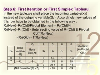
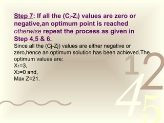
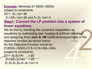
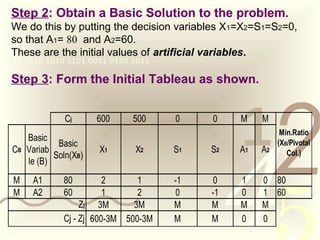
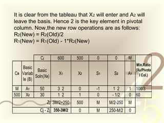
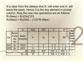
This document provides an overview of linear programming problems and methods for solving them. It defines a linear programming problem and describes how to write it in standard form with decision variables and constraints. It then explains the simplex method, including how to form an initial tableau and iterate to reach an optimal solution. Finally, it introduces the Big-M method for handling problems with inequality constraints by adding artificial variables with large penalty coefficients. An example demonstrates both simplex and Big-M methods.

1. 421
0011 0010 1010 1101 0001 0100 1011
Solving Linear
Programming Problems
Shubhagata Roy

2. 421
0011 0010 1010 1101 0001 0100 1011
Q. What is a Linear Programming Problem?
A. A Linear Programming Problem(LPP) is a problem in
which we are asked to find the maximum (or minimum) value
of a linear objective function
Z = aX1 + bX2 + cX2 + ... (e.g. Z = 3X1 + 2X2 + X3)
Subject to one or more linear constraints of the form
AX1+ BX2 + CX3 + . . <or= N (e.g. X1 + X2 + 3X3 <or= 12)
The desired largest (or smallest) value of the objective
function is called the optimal value, and a collection of values
of X1,X2,X3, . . . that gives the optimal value constitutes an
optimal solution.The variables X1, X2, X3, . . are called the
decision variables.

3. 421
0011 0010 1010 1101 0001 0100 1011
Simplex Method
The most frequently used method to solve LP problems is the
Simplex Method. Before going into the method, we must get
familiarized with some important terminologies :
Standard Form- A linear program in which all the constraints
are written as equalities.
Slack Variable- A variable added to the LHS of “Less than or
equal to” constraint to convert it into an equality.
Surplus Variable- A variable subtracted from the LHS of
“More than or equal to” constraint to convert it into an equality.
Basic Solution- For a system of m linear equations in n
variables (n>m),a solution obtained by setting (n-m) variables
equal to zero and solving the system of equations for
remaining m variables.
Basic Feasible Solution(BFS)- If all the variables in basic
solution are more than or equal to zero.

4. 421
0011 0010 1010 1101 0001 0100 1011
Optimum Solution- Any BFS which optimizes(maximizes
or minimizes) the objective function.
Tableau Form- When a LPP is written in a tabular form
prior to setting up the Initial Simplex Tableau.
Simplex Tableau- A table which is used to keep track of
the calculations made at each iteration when the simplex
method is employed.
Net EvaluationRow(Cj-Zj )- The row containing net profit or
loss.The nos.in this row are also known as shadow prices.
Pivotal Column- The column having largest positive(or
negative) value in the Net Evaluation Row for a
maximization(or minimization) problem.
Pivotal Row- The row corresponding to variable that will
leave the table in order to make room for another variable.
Pivotal Element- Element at the intersection of pivotal row
and pivotal column.

5. 421
0011 0010 1010 1101 0001 0100 1011
To understand the method,let us take an example
containing two decision variables and two constraints.
Example:
Maximize Z = 7X1+5X2 , subject to the constraints,
X1+2X2 < or = 6
4X1+3X2 < or = 12 and X1 & X2 are non-negative.
Step1: Convert the LP problem into a system of
linear equations.
We do this by rewriting the constraint inequalities as
equations by adding new "slack variables" and assigning
them zero coefficients(profits) in the objective function as
shown below:
X1+2X2+S1 = 6
4X1+3X2 +S2 = 12
And the Objective Function would be:
Z=7X1+5X2+0.S1+0.S2

6. 421
0011 0010 1010 1101 0001 0100 1011
Step 2: Obtain a Basic Solution to the problem.
We do this by putting the decision variables X1=X2=0,
so that
S1= 6 and S2=12.
These are the initial values of slack variables.
Step 3: Form the Initial Tableau as shown.
Cj 7 5 0 0
CB
Basic
Variable
(B)
Basic
Soln(XB)
X1 X2 S1 S2
0 S1 6 1 2 1 0 6/1=6
0 S2 12 4 3 0 1 12/4=3
0 0 0 0
7 5 0 0
Initial Tableau
Min.Ratio
(XB/Pivotal
Col.)
Zj
(Net Evaluation)Cj - Zj

7. 421
0011 0010 1010 1101 0001 0100 1011Step 4: Find (Cj-Zj) having highest positive value.
The column corresponding to this value,is called the Pivotal
Column and enters the table. In the previous table,column
corresponding to variable X1 is the pivotal column.
Step 5: Find the Minimum Positive Ratio.
Divide XB values by the corresponding values of Pivotal
Column.The row corresponding to the minimum positive
value is the Pivotal Row and leaves the table. In the
previous table,row corresponding to the slack variable S2 is
the pivotal row.

8. 421
0011 0010 1010 1101 0001 0100 1011
Step 6: First Iteration or First Simplex Tableau.
In the new table,we shall place the incoming variable(X1)
instead of the outgoing variable(S2). Accordingly,new values of
this row have to be obtained in the following way :
R2(New)=R2(Old)/Pivotal Element = R2(Old)/4
R1(New)=R1(Old) - (Intersecting value of R1(Old) & Pivotal
Col)*R2(New)
=R1(Old) - 1*R2(New)
Cj 7 5 0 0
CB
Basic
Variable
(B)
Basic
Soln(XB)
X1 X2 S1 S2
0 S1 3 0 5 4 1 - 1/4
7 X1 3 1 3/4 0 1/4
7 21 4 0 7 4
0 - 1/4 0 -74
Zj
(Net Evaluation)Cj - Zj
Min.Ratio
(XB/Pivotal
Col.)

9. 421
0011 0010 1010 1101 0001 0100 1011
Step 7: If all the (Cj-Zj) values are zero or
negative,an optimum point is reached
otherwise repeat the process as given in
Step 4,5 & 6.
Since all the (Cj-Zj) values are either negative or
zero,hence an optimum solution has been achieved.The
optimum values are:
X1=3,
X2=0 and,
Max Z=21.

10. 421
0011 0010 1010 1101 0001 0100 1011
Big-M Method of solving LPP
The Big-M method of handling instances with artificial
variables is the “commonsense approach”. Essentially, the
notion is to make the artificial variables, through their
coefficients in the objective function, so costly or unprofitable
that any feasible solution to the real problem would be
preferred....unless the original instance possessed no feasible
solutions at all. But this means that we need to assign, in the
objective function, coefficients to the artificial variables that are
either very small (maximization problem) or very large
(minimization problem); whatever this value,let us call it Big M.
In fact, this notion is an old trick in optimization in general; we
simply associate a penalty value with variables that we do not
want to be part of an ultimate solution(unless such an outcome
Is unavoidable).

11. 421
0011 0010 1010 1101 0001 0100 1011
Indeed, the penalty is so costly that unless any of the
respective variables' inclusion is warranted algorithmically,
such variables will never be part of any feasible solution.
This method removes artificial variables from the basis. Here,
we assign a large undesirable (unacceptable penalty)
coefficients to artificial variables from the objective function
point of view. If the objective function (Z) is to be minimized,
then a very large positive price (penalty, M) is assigned to
each artificial variable and if Z is to be minimized, then a very
large negative price is to be assigned. The penalty will be
designated by +M for minimization problem and by –M for a
maximization problem and also M>0.

12. 421
0011 0010 1010 1101 0001 0100 1011
Example: Minimize Z= 600X1+500X2
subject to constraints,
2X1+ X2 >or= 80
X1+2X2 >or= 60 and X1,X2 >or= 0
Step1: Convert the LP problem into a system of
linear equations.
We do this by rewriting the constraint inequalities as
equations by subtracting new “surplus & artificial variables"
and assigning them zero & +M coefficientsrespectively in the
objective function as shown below.
So the Objective Function would be:
Z=600X1+500X2+0.S1+0.S2+MA1+MA2
subject to constraints,
2X1+ X2-S1+A1 = 80
X1+2X2-S2+A2 = 60
X1,X2,S1,S2,A1,A2 >or= 0

13. 421
0011 0010 1010 1101 0001 0100 1011
Step 2: Obtain a Basic Solution to the problem.
We do this by putting the decision variables X1=X2=S1=S2=0,
so that A1= 80 and A2=60.
These are the initial values of artificial variables.
Step 3: Form the Initial Tableau as shown.
Cj 600 500 0 0 M M
CB
Basic
Variab
le (B)
Basic
Soln(XB)
X1 X2 S1 S2 A1 A2
M A1 80 2 1 -1 0 1 0 80
M A2 60 1 2 0 -1 0 1 60
3M 3M M M M M
600-3M 500-3M M M 0 0
Min.Ratio
(XB/Pivotal
Col.)
Zj
Cj - Zj

14. 421
0011 0010 1010 1101 0001 0100 1011
It is clear from the tableau that X2 will enter and A2 will
leave the basis. Hence 2 is the key element in pivotal
column. Now,the new row operations are as follows:
R2(New) = R2(Old)/2
R1(New) = R1(Old) - 1*R2(New)
Cj 600 500 0 0 M
CB
Basic
Variab
le (B)
Basic
Soln(XB)
X1 X2 S1 S2 A1
M A1 50 3 2 0 -1 1 2 1 100/3
500 X2 30 1 2 1 0 - 1/2 0 60
3M/2+250 500 M M/2-250 M
350-3M/2 0 M 250-M/2 0
Min.Ratio
(XB/Pivota
l Col.)
Zj
Cj - Zj

15. 421
0011 0010 1010 1101 0001 0100 1011
It is clear from the tableau that X1 will enter and A1 will
leave the basis. Hence 2 is the key element in pivotal
column. Now,the new row operations are as follows:
R1(New) = R1(Old)*2/3
R2(New) = R2(Old) – (1/2)*R1(New)
Cj 600 500 0 0
CB
Basic
Varia
ble
(B)
Basic
Soln(XB)
X1 X2 S1 S2
600 X1 100/3 1 0 2 3 1 3
500 X2 40/3 0 1 1 3 2 3
600 500 700 3 400 3
0 0 700 3 400 3
Zj
Cj - Zj
Min.
Ratio
(XB/P
ivotal
Col.)

16. 421
0011 0010 1010 1101 0001 0100 1011
Since all the values of (Cj-Zj) are either zero or positive
and also both the artificial variables have been removed,
an optimum solution has been arrived at with X1=100/3 ,
X2=40/3 and Z=80,000/3.

17. 421
0011 0010 1010 1101 0001 0100 1011