Download as PDF, PPTX
![LINEAR PROGRAMMING: ITERATIVE METHODS
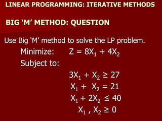
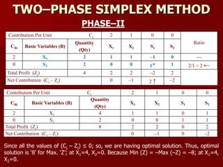
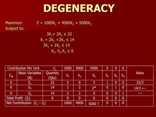
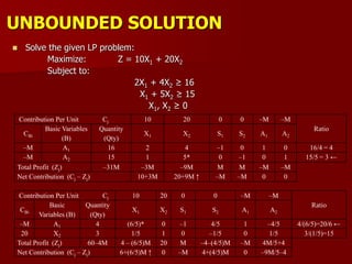
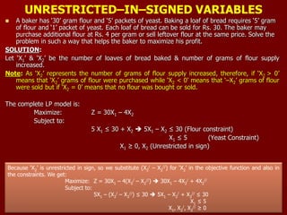
Standard LP Form:
Maximize: Z = 160X1 + 200X2 + 0S1 + 0S2 + 0S3
Subject to:
2X1 + 4X2 + S1 = 40
18X1 + 18X2 + S2 = 216
24X1 + 12X2 + S3 = 240
X1, X2, S1, S2, S3 ≥ 0
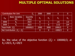
Contribution Per Unit Cj 160 200 0 0
0
Ratio = [Qty / PE > 0]
CBi
Basic Variables
(B)
Quantity
(Qty)
X1 X2 S1 S2 S3
0 S1 40 2 4* 1 0 0 40/4 = 10 ←
0 S2 216 18 18 0 1 0 216/18 = 12
0 S3 240 24 12 0 0 1 240/12 = 20
Total Profit (Zj) 0 0 0 0 0 0
Net Contribution (Cj – Zj) 160 200 ↑ 0 0
0](https://image.slidesharecdn.com/2-150928162159-lva1-app6891/85/2-lp-iterative-methods-6-320.jpg)
![LINEAR PROGRAMMING: ITERATIVE METHODS
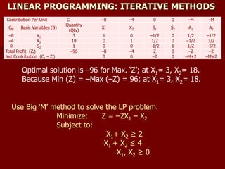
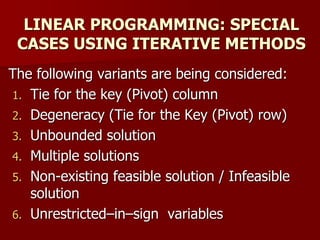
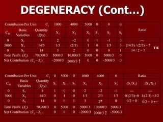
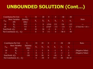
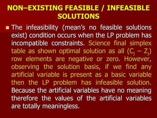
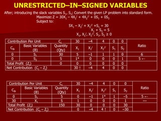
Contribution Per Unit Cj 160 200 0 0 0
CBi
Basic Variables
(B)
Quantity
(Qty)
X1 X2 S1 S2 S3
200 X2 8 0 1 1/2 –1/18 0
160 X1 4 1 0 –1/2 1/9 0
0 S3 48 0 0 6 –2 1
Total Profit (Zj) 2240 160 200 20 20/3 0
Net Contribution (Cj – Zj) 0 0 –20 –20/3 0
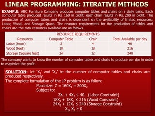
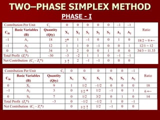
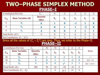
Since all the values of (Cj – Zj) ≤ 0; so, the solution is optimal. Optimal solution is
2240 for Max. ‘Z’; at X1= 4, X2= 8.
Contribution Per Unit Cj 160 200 0 0 0
Ratio = [Qty / PE > 0]
CBi
Basic Variables
(B)
Quantity
(Qty)
X1 X2 S1 S2 S3
200 X2 10 1/2 1 1/4 0 0 10/(1/2) = 20
0 S2 36 9* 0 –9/2 1 0 36/9 = 4 ←
0 S3 120 18 0 –3 0 1 120/18 = 20/3
Total Profit (Zj) 2000 100 200 50 0 0
Net Contribution (Cj – Zj) 60 ↑ 0 –50 0 0](https://image.slidesharecdn.com/2-150928162159-lva1-app6891/85/2-lp-iterative-methods-7-320.jpg)
![LINEAR PROGRAMMING: ITERATIVE METHODS
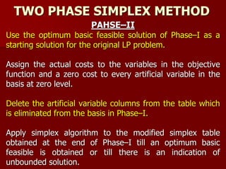
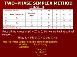
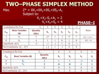
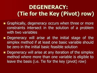
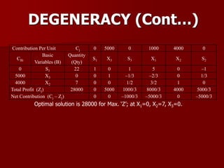
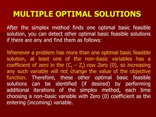
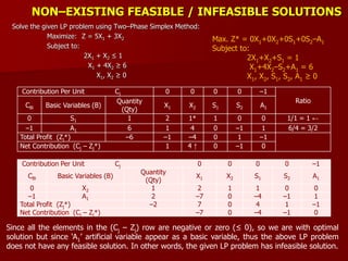
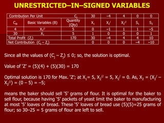
Maximize: Z = –8X1 –4X2 + 0S1 + 0S2 – MA1 – MA2
Subject to:
3X1+ X2–S1+A1 = 27
X1+ X2+A2 = 21
X1+2X2+S2 = 40
X1, X2, S1, S2, A1, A2 ≥ 0
Contribution Per Unit Cj –8 –4 0 0 –M –M
Ratio=
[Qty/PE>0]CBi
Basic Variables
(B)
Quantity
(Qty)
X1 X2 S1 S2 A1 A2
–M A1 27 3* 1 –1 0 1 0 27/3 = 9 ←
–M A2 21 1 1 0 0 0 1 21/1 = 21
0 S2 40 1 2 0 1 0 0 40/1 = 40
Total Profit (Zj) –48M –4M –2M M 0 –M –M
Net Contribution (Cj – Zj) –8+4M ↑ –4+2M –M 0 0 0
Contribution Per Unit
Cj
–8 –4 0 0 –M –M
Ratio
CBi
Basic
Variables (B)
Quantity
(Qty)
X1 X2 S1 S2 A1 A2
–8 X1 9 1 1/3 –1/3 0 1/3 0 27
–M A2 12 0 (2/3)* 1/3 0 –1/3 1 18 ←
0 S2 31 0 5/3 1/3 1 –1/3 0 18.6
Total Profit (Zj) –72–12M –8 –8/3–(2/3)M 8/3–M/3 0 –8/3+M/3 –M
Net Contribution (Cj – Zj) 0 –4/3+(2/3)M
↑
–8/3+M/3 0 8/3– (2/3)M 0](https://image.slidesharecdn.com/2-150928162159-lva1-app6891/85/2-lp-iterative-methods-9-320.jpg)


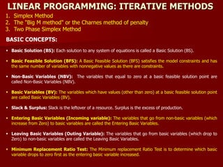
This document discusses linear programming iterative methods. It introduces the simplex method, two-phase simplex method, and Big M method. An example problem is provided to illustrate solving a linear programming problem using these iterative methods. The problem involves maximizing profit from producing tables and chairs given resource constraints. The problem is formulated and solved using the simplex method in multiple steps.