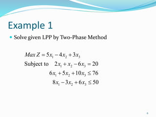
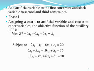
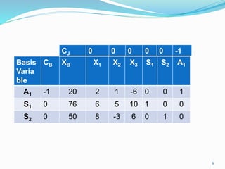
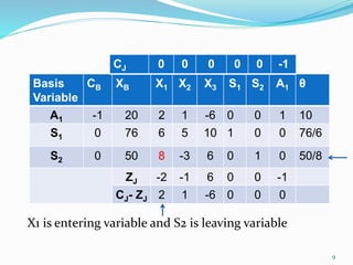
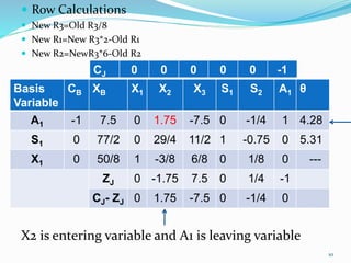
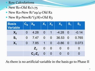
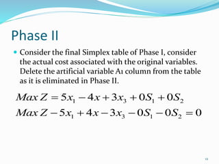
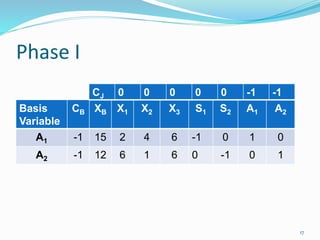
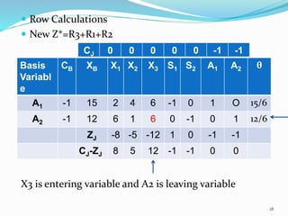
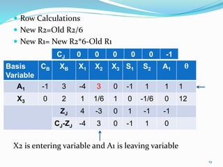
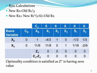
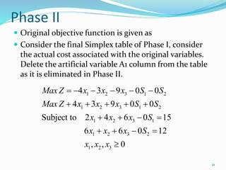
SlideShare a Scribd company logo
Linear Programming
Two Phase Method
1
Two Phase Method
 For greater than or equal to constraint, the
slack variable has a negative co efficient
 Equality constraints do not have slack
variables
 If either of constraint is part of the model,
there is no convenient IBFS and hence two
phase method is used
2
Phase I
1. In this phase, we find an IBFS to the original
problem, for this all artificial variable are to be driven
to zero. To do this an artificial objective function (Z*)
is created which is the sum of all artificial variables.
The new objective function is then subjected to the
constraints of the given original problem using the
simplex method. At the end of Phase I, three cases
arises
A. If the minimum value of Z*=0, and no artificial
variable appears in the basis at a positive level then
the given problem has no feasible solution and
procedure terminates.
3
B. If the minimum value of Z*=0, and no artificial
variable appears in the basis, then a basic feasible
solution to the given problem is obtained.
C. If the minimum value of the Z*=0 and one or
more artificial variable appears in the basis at
zero level, then a feasible solution to the original
problem is obtained. However, we must take care
of this artificial variable and see that it never
become positive during Phase II computations.
4
Phase II
 When Phase I results in (B) or (C), we go on for Phase
II to find optimum solution to the given LP problem.
The basic feasible solution found at the end of Phase I
now used as a starting solution for the original LP
problem. Mean that find table of Phase I becomes
initial table for Phase II in which artificial (auxiliary)
objective function is replaced by the original objective
function. Simplex method is then applied to arrive at
optimum solution.
5
Example 1
 Solve given LPP by Two-Phase Method
1 2 3
1 2 3
1 2 3
1 2 3
5 4 3
Subject to 2 6 20
6 5 10 76
8 3 6 50
Max Z x x x
x x x
x x x
x x x
  
  
  
  
6
 Add artificial variable to the first constraint and slack
variable to second and third constraints.
 Phase I
 Assigning a cost 1 to artificial variable and cost o to
other variables, the objective function of the auxiliary
LPP is
1 2 3 1
1 2 3 1
1 2 3 1
1 2 3 1
1 2 3 2
* 0 0 0
* 0 0 0 0
Subject to 2 6 20
6 5 10 76
8 3 6 50
MinZ x x x A
MinZ x x x A
x x x A
x x x S
x x x S
   
    
   
   
   
7
-Max
Basis
Varia
ble
CB XB X1 X2 X3 S1 S2 A1
A1 -1 20 2 1 -6 0 0 1
S1 0 76 6 5 10 1 0 0
S2 0 50 8 -3 6 0 1 0
8
CJ 0 0 0 0 0 -1
X1 is entering variable and S2 is leaving variable
Basis
Variable
CB XB X1 X2 X3 S1 S2 A1 θ
A1 -1 20 2 1 -6 0 0 1 10
S1 0 76 6 5 10 1 0 0 76/6
S2 0 50 8 -3 6 0 1 0 50/8
ZJ -2 -1 6 0 0 -1
CJ- ZJ 2 1 -6 0 0 0
9
CJ 0 0 0 0 0 -1
 Row Calculations
 New R3=Old R3/8
 New R1=New R3*2-Old R1
 New R2=NewR3*6-Old R2
 X2 is entering variable and A1 is leaving variable
Basis
Variable
CB XB X1 X2 X3 S1 S2 A1 θ
A1 -1 7.5 0 1.75 -7.5 0 -1/4 1 4.28
S1 0 77/2 0 29/4 11/2 1 -0.75 0 5.31
X1 0 50/8 1 -3/8 6/8 0 1/8 0 ---
ZJ 0 -1.75 7.5 0 1/4 -1
CJ- ZJ 0 1.75 -7.5 0 -1/4 0
10
CJ 0 0 0 0 0 -1
X2 is entering variable and A1 is leaving variable
 Row Calculations
 New R1=Old R1/1.75
 New R2=New R1*29/4-Old R2
 New R3=NewR1*(3/8)+Old R3
As there is no artificial variable in the basis go to Phase II
Basis
Variable
CB XB X1 X2 X3 S1 S2
X2 0 4.28 0 1 -4.28 0 -0.14
S1 0 7.47 0 0 36.53 0 0.765
X1 0 7.85 1 0 -0.86 0 0.073
ZJ 0 0 0 0 0
CJ-ZJ 0 0 0 0 0
11
Phase II
 Consider the final Simplex table of Phase I, consider
the actual cost associated with the original variables.
Delete the artificial variable A1 column from the table
as it is eliminated in Phase II.
1 3 1 2
1 3 1 2
5 4 3 0 0
5 4 3 0 0 0
Max Z x x x S S
Max Z x x x S S
    
     
12
Basis
Variable
CB XB X1 X2 X3 S1 S2
X2 -4 4.28 0 1 -4.28 0 -0.14
S1 0 7.47 0 0 36.53 0 0.765
X1 5 7.85 1 0 -0.86 0 0.073
ZJ 5 -4 12.82 0 0.925
CJ-ZJ 0 0 -9.82 0 -0.925
13
CJ 5 -4 3 0 0
 As the given problem is of maximization and all the
values in CJ-ZJ row are either zero or negative, an
optimal solution is reached and is given by
 X1=7.855
 X2=4.28 and
 Z=5X1-4X2+3X3
 Z=5(7.855)-4(4.28)+3(0)
= 22.15
14
Example 2
 Solve by Two-Phase Simplex Method
1 2 3
1 2 3
1 2 3
1 2 3
4 3 9
Subject to 2 4 6 15
6 6 12
, , 0
Max Z x x x
x x x
x x x
x x x
   
  
  

15
 Add artificial variable to the first constraint and slack
variable to second and third constraints.
 Phase I
 Assigning a cost 1 to artificial variable and cost o to
other variables, the objective function of the auxiliary
LPP is
A new auxiliary linear programming problem
16
1 2 3 1 2
1 2
1 2 3 1 1
1 2 3 2 2
* 0 0 0
* 0
2 4 6 15
6 6 12
Min Z x x x A A
Min Z A A
x x x S A
x x x S A
    
  
    
    
Max - -
Phase I
Basis
Variable
CB XB X1 X2 X3 S1 S2 A1 A2
A1 -1 15 2 4 6 -1 0 1 0
A2 -1 12 6 1 6 0 -1 0 1
17
CJ 0 0 0 0 0 -1 -1
 Row Calculations
 New Z*=R3+R1+R2
X3 is entering variable and A2 is leaving variable
Basis
Variabl
e
CB XB X1 X2 X3 S1 S2 A1 A2 θ
A1 -1 15 2 4 6 -1 0 1 O 15/6
A2 -1 12 6 1 6 0 -1 0 1 12/6
ZJ -8 -5 -12 1 0 -1 -1
CJ-ZJ 8 5 12 -1 -1 0 0
18
CJ 0 0 0 0 0 -1 -1
 Row Calculations
 New R2=Old R2/6
 New R1= New R2*6-Old R1
X2 is entering variable and A1 is leaving variable
Basis
Variable
CB XB X1 X2 X3 S1 S2 A1 θ
A1 -1 3 -4 3 0 -1 1 1 1
X3 0 2 1 1/6 1 0 -1/6 0 12
ZJ 4 -3 0 1 -1 -1
CJ-ZJ -4 3 0 -1 1 0
19
CJ 0 0 0 0 0 -1
 Row Calculations
 New R1=Old R1/3
 New R2= New R1*(1/6)-Old R2
Optimality condition is satisfied as Z* is having zero
value
Basis
Variable
CB XB X1 X2 X3 S1 S2
X2 0 1 -4/3 1 0 -1/3 1/3
X3 0 11/6 11/9 0 1 1/18 -2/9
ZJ 0 0 0 0 0
CJ-ZJ 0 0 0 0 0
20
CJ 0 0 0 0 0
Phase II
 Original objective function is given as
 Consider the final Simplex table of Phase I, consider
the actual cost associated with the original variables.
Delete the artificial variable A1 column from the table
as it is eliminated in Phase II.
1 2 3 1 2
1 2 3 1 2
1 2 3 1
1 2 3 2
1 2 3
4 3 9 0 0
4 3 9 0 0
Subject to 2 4 6 0 15
6 6 0 12
, , 0
Max Z x x x S S
Max Z x x x S S
x x x S
x x x S
x x x
     
    
   
   

21
Initial Basic Feasible Solution
Basis
Variable
CB XB X1 X2 X3 S1 S2 θ
X2 -3 1 -4/3 1 0 -1/3 1/3 9/4
X3 -9 11/6 11/9 0 1 1/18 -2/9 1.5
ZJ -7 -3 -9 -1/2 -1
CJ-ZJ 3 0 0 1/2 1
22
CJ -4 -3 -9 0 0
X1 is entering variable and X3 is leaving variable
 Row Calculations
 New R2=Old R2/(11/9)
 New R1=New R2+Old R1
 As all the values in Z row are zero or negative, the
condition of optimality is reached.
Basis
Variable
CB XB X1 X2 X3 S1 S2
X2 -3 3 0 1 12/11 -3/11 13/33
X1 -4 3/2 1 0 9/11 1/22 -2/11
ZJ -4 -3 72/11 7/11 3/11
CJ-ZJ 0 0 -27/11 -7/11 -3/11
23
CJ -4 -3 -9 0 0
 X1=3/2
 X3=3
 Hence Z= -4X1 -3X2 -9X3
Z= -4(1.5)-3(3)-9(0)
Z= -15
24
Thank You
25

More Related Content

What's hot

Simplex method concept,
Simplex method concept,Simplex method concept,
Simplex method concept,
Dronak Sahu
 
Graphical Method
Graphical MethodGraphical Method
Graphical Method
Sachin MK
 

What's hot (20)

Simplex method concept,
Simplex method concept,Simplex method concept,
Simplex method concept,
 
Chapter 4 Simplex Method ppt
Chapter 4  Simplex Method pptChapter 4  Simplex Method ppt
Chapter 4 Simplex Method ppt
 
Simplex Algorithm
Simplex AlgorithmSimplex Algorithm
Simplex Algorithm
 
Operation Research (Simplex Method)
Operation Research (Simplex Method)Operation Research (Simplex Method)
Operation Research (Simplex Method)
 
Sensitivity analysis linear programming copy
Sensitivity analysis linear programming   copySensitivity analysis linear programming   copy
Sensitivity analysis linear programming copy
 
Operation research - the revised simplex method
Operation research - the revised simplex methodOperation research - the revised simplex method
Operation research - the revised simplex method
 
Operations Research - The Dual Simplex Method
Operations Research - The Dual Simplex MethodOperations Research - The Dual Simplex Method
Operations Research - The Dual Simplex Method
 
Simplex Method
Simplex MethodSimplex Method
Simplex Method
 
The Big M Method - Operation Research
The Big M Method - Operation ResearchThe Big M Method - Operation Research
The Big M Method - Operation Research
 
Duality in Linear Programming
Duality in Linear ProgrammingDuality in Linear Programming
Duality in Linear Programming
 
Operation research unit 1: LPP Big M and Two Phase method
Operation research unit 1: LPP Big M and Two Phase methodOperation research unit 1: LPP Big M and Two Phase method
Operation research unit 1: LPP Big M and Two Phase method
 
Special Cases in Simplex Method
Special Cases in Simplex MethodSpecial Cases in Simplex Method
Special Cases in Simplex Method
 
Graphical Method
Graphical MethodGraphical Method
Graphical Method
 
Linear Programming
Linear ProgrammingLinear Programming
Linear Programming
 
LINEAR PROGRAMMING
LINEAR PROGRAMMINGLINEAR PROGRAMMING
LINEAR PROGRAMMING
 
Simplex method
Simplex methodSimplex method
Simplex method
 
Duality in Linear Programming Problem
Duality in Linear Programming ProblemDuality in Linear Programming Problem
Duality in Linear Programming Problem
 
Linear Programming (graphical method)
Linear Programming (graphical method)Linear Programming (graphical method)
Linear Programming (graphical method)
 
Stepping Stone Method
Stepping Stone MethodStepping Stone Method
Stepping Stone Method
 
Simplex Method Explained
Simplex Method ExplainedSimplex Method Explained
Simplex Method Explained
 

Similar to Two Phase Method- Linear Programming

Twophasemethod 131003081339-phpapp01
Twophasemethod 131003081339-phpapp01Twophasemethod 131003081339-phpapp01
Twophasemethod 131003081339-phpapp01
kongara
 
Simplex method - Maximisation Case
Simplex method - Maximisation CaseSimplex method - Maximisation Case
Simplex method - Maximisation Case
Joseph Konnully
 
OR Linear Programming
OR Linear ProgrammingOR Linear Programming
OR Linear Programming
chaitu87
 

Similar to Two Phase Method- Linear Programming (20)

Twophasemethod 131003081339-phpapp01
Twophasemethod 131003081339-phpapp01Twophasemethod 131003081339-phpapp01
Twophasemethod 131003081339-phpapp01
 
Linear programming
Linear programmingLinear programming
Linear programming
 
Simplex two phase
Simplex two phaseSimplex two phase
Simplex two phase
 
Simplex algorithm
Simplex algorithmSimplex algorithm
Simplex algorithm
 
simplex method-maths 4 mumbai university
simplex method-maths 4 mumbai universitysimplex method-maths 4 mumbai university
simplex method-maths 4 mumbai university
 
2. lp iterative methods
2. lp   iterative methods2. lp   iterative methods
2. lp iterative methods
 
Operations research 1_the_two-phase_simp
Operations research 1_the_two-phase_simpOperations research 1_the_two-phase_simp
Operations research 1_the_two-phase_simp
 
Simplex part 2 of 4
Simplex part 2 of 4Simplex part 2 of 4
Simplex part 2 of 4
 
MFCS2-Module1.pptx
MFCS2-Module1.pptxMFCS2-Module1.pptx
MFCS2-Module1.pptx
 
Lp model, simplex method
Lp model, simplex method   Lp model, simplex method
Lp model, simplex method
 
Chapter four
Chapter fourChapter four
Chapter four
 
Simplex method - Maximisation Case
Simplex method - Maximisation CaseSimplex method - Maximisation Case
Simplex method - Maximisation Case
 
Ouantitative technics
Ouantitative technics Ouantitative technics
Ouantitative technics
 
aaoczc2252
aaoczc2252aaoczc2252
aaoczc2252
 
SG 8 Lecture 15 Simplex - Min - 2 phase.pptx
SG 8 Lecture 15 Simplex - Min - 2 phase.pptxSG 8 Lecture 15 Simplex - Min - 2 phase.pptx
SG 8 Lecture 15 Simplex - Min - 2 phase.pptx
 
Simplex method
Simplex methodSimplex method
Simplex method
 
OR Linear Programming
OR Linear ProgrammingOR Linear Programming
OR Linear Programming
 
Integer Linear Programming
Integer Linear ProgrammingInteger Linear Programming
Integer Linear Programming
 
Linear programming
Linear programmingLinear programming
Linear programming
 
Applied numerical methods lec6
Applied numerical methods lec6Applied numerical methods lec6
Applied numerical methods lec6
 

Recently uploaded

Fruit shop management system project report.pdf
Fruit shop management system project report.pdfFruit shop management system project report.pdf
Fruit shop management system project report.pdf
Kamal Acharya
 
Hall booking system project report .pdf
Hall booking system project report  .pdfHall booking system project report  .pdf
Hall booking system project report .pdf
Kamal Acharya
 
Online blood donation management system project.pdf
Online blood donation management system project.pdfOnline blood donation management system project.pdf
Online blood donation management system project.pdf
Kamal Acharya
 
Standard Reomte Control Interface - Neometrix
Standard Reomte Control Interface - NeometrixStandard Reomte Control Interface - Neometrix
Standard Reomte Control Interface - Neometrix
Neometrix_Engineering_Pvt_Ltd
 
Laundry management system project report.pdf
Laundry management system project report.pdfLaundry management system project report.pdf
Laundry management system project report.pdf
Kamal Acharya
 

Recently uploaded (20)

Fruit shop management system project report.pdf
Fruit shop management system project report.pdfFruit shop management system project report.pdf
Fruit shop management system project report.pdf
 
A CASE STUDY ON ONLINE TICKET BOOKING SYSTEM PROJECT.pdf
A CASE STUDY ON ONLINE TICKET BOOKING SYSTEM PROJECT.pdfA CASE STUDY ON ONLINE TICKET BOOKING SYSTEM PROJECT.pdf
A CASE STUDY ON ONLINE TICKET BOOKING SYSTEM PROJECT.pdf
 
Pharmacy management system project report..pdf
Pharmacy management system project report..pdfPharmacy management system project report..pdf
Pharmacy management system project report..pdf
 
HYDROPOWER - Hydroelectric power generation
HYDROPOWER - Hydroelectric power generationHYDROPOWER - Hydroelectric power generation
HYDROPOWER - Hydroelectric power generation
 
Online resume builder management system project report.pdf
Online resume builder management system project report.pdfOnline resume builder management system project report.pdf
Online resume builder management system project report.pdf
 
Furniture showroom management system project.pdf
Furniture showroom management system project.pdfFurniture showroom management system project.pdf
Furniture showroom management system project.pdf
 
Introduction to Machine Learning Unit-4 Notes for II-II Mechanical Engineering
Introduction to Machine Learning Unit-4 Notes for II-II Mechanical EngineeringIntroduction to Machine Learning Unit-4 Notes for II-II Mechanical Engineering
Introduction to Machine Learning Unit-4 Notes for II-II Mechanical Engineering
 
Electrostatic field in a coaxial transmission line
Electrostatic field in a coaxial transmission lineElectrostatic field in a coaxial transmission line
Electrostatic field in a coaxial transmission line
 
Hall booking system project report .pdf
Hall booking system project report  .pdfHall booking system project report  .pdf
Hall booking system project report .pdf
 
Top 13 Famous Civil Engineering Scientist
Top 13 Famous Civil Engineering ScientistTop 13 Famous Civil Engineering Scientist
Top 13 Famous Civil Engineering Scientist
 
Introduction to Machine Learning Unit-5 Notes for II-II Mechanical Engineering
Introduction to Machine Learning Unit-5 Notes for II-II Mechanical EngineeringIntroduction to Machine Learning Unit-5 Notes for II-II Mechanical Engineering
Introduction to Machine Learning Unit-5 Notes for II-II Mechanical Engineering
 
Introduction to Casting Processes in Manufacturing
Introduction to Casting Processes in ManufacturingIntroduction to Casting Processes in Manufacturing
Introduction to Casting Processes in Manufacturing
 
Online blood donation management system project.pdf
Online blood donation management system project.pdfOnline blood donation management system project.pdf
Online blood donation management system project.pdf
 
Standard Reomte Control Interface - Neometrix
Standard Reomte Control Interface - NeometrixStandard Reomte Control Interface - Neometrix
Standard Reomte Control Interface - Neometrix
 
Laundry management system project report.pdf
Laundry management system project report.pdfLaundry management system project report.pdf
Laundry management system project report.pdf
 
KIT-601 Lecture Notes-UNIT-4.pdf Frequent Itemsets and Clustering
KIT-601 Lecture Notes-UNIT-4.pdf Frequent Itemsets and ClusteringKIT-601 Lecture Notes-UNIT-4.pdf Frequent Itemsets and Clustering
KIT-601 Lecture Notes-UNIT-4.pdf Frequent Itemsets and Clustering
 
ONLINE CAR SERVICING SYSTEM PROJECT REPORT.pdf
ONLINE CAR SERVICING SYSTEM PROJECT REPORT.pdfONLINE CAR SERVICING SYSTEM PROJECT REPORT.pdf
ONLINE CAR SERVICING SYSTEM PROJECT REPORT.pdf
 
Democratizing Fuzzing at Scale by Abhishek Arya
Democratizing Fuzzing at Scale by Abhishek AryaDemocratizing Fuzzing at Scale by Abhishek Arya
Democratizing Fuzzing at Scale by Abhishek Arya
 
KIT-601 Lecture Notes-UNIT-5.pdf Frame Works and Visualization
KIT-601 Lecture Notes-UNIT-5.pdf Frame Works and VisualizationKIT-601 Lecture Notes-UNIT-5.pdf Frame Works and Visualization
KIT-601 Lecture Notes-UNIT-5.pdf Frame Works and Visualization
 
RESORT MANAGEMENT AND RESERVATION SYSTEM PROJECT REPORT.pdf
RESORT MANAGEMENT AND RESERVATION SYSTEM PROJECT REPORT.pdfRESORT MANAGEMENT AND RESERVATION SYSTEM PROJECT REPORT.pdf
RESORT MANAGEMENT AND RESERVATION SYSTEM PROJECT REPORT.pdf
 

Two Phase Method- Linear Programming

  • 2. Two Phase Method  For greater than or equal to constraint, the slack variable has a negative co efficient  Equality constraints do not have slack variables  If either of constraint is part of the model, there is no convenient IBFS and hence two phase method is used 2
  • 3. Phase I 1. In this phase, we find an IBFS to the original problem, for this all artificial variable are to be driven to zero. To do this an artificial objective function (Z*) is created which is the sum of all artificial variables. The new objective function is then subjected to the constraints of the given original problem using the simplex method. At the end of Phase I, three cases arises A. If the minimum value of Z*=0, and no artificial variable appears in the basis at a positive level then the given problem has no feasible solution and procedure terminates. 3
  • 4. B. If the minimum value of Z*=0, and no artificial variable appears in the basis, then a basic feasible solution to the given problem is obtained. C. If the minimum value of the Z*=0 and one or more artificial variable appears in the basis at zero level, then a feasible solution to the original problem is obtained. However, we must take care of this artificial variable and see that it never become positive during Phase II computations. 4
  • 5. Phase II  When Phase I results in (B) or (C), we go on for Phase II to find optimum solution to the given LP problem. The basic feasible solution found at the end of Phase I now used as a starting solution for the original LP problem. Mean that find table of Phase I becomes initial table for Phase II in which artificial (auxiliary) objective function is replaced by the original objective function. Simplex method is then applied to arrive at optimum solution. 5
  • 6. Example 1  Solve given LPP by Two-Phase Method 1 2 3 1 2 3 1 2 3 1 2 3 5 4 3 Subject to 2 6 20 6 5 10 76 8 3 6 50 Max Z x x x x x x x x x x x x             6
  • 7.  Add artificial variable to the first constraint and slack variable to second and third constraints.  Phase I  Assigning a cost 1 to artificial variable and cost o to other variables, the objective function of the auxiliary LPP is 1 2 3 1 1 2 3 1 1 2 3 1 1 2 3 1 1 2 3 2 * 0 0 0 * 0 0 0 0 Subject to 2 6 20 6 5 10 76 8 3 6 50 MinZ x x x A MinZ x x x A x x x A x x x S x x x S                      7 -Max
  • 8. Basis Varia ble CB XB X1 X2 X3 S1 S2 A1 A1 -1 20 2 1 -6 0 0 1 S1 0 76 6 5 10 1 0 0 S2 0 50 8 -3 6 0 1 0 8 CJ 0 0 0 0 0 -1
  • 9. X1 is entering variable and S2 is leaving variable Basis Variable CB XB X1 X2 X3 S1 S2 A1 θ A1 -1 20 2 1 -6 0 0 1 10 S1 0 76 6 5 10 1 0 0 76/6 S2 0 50 8 -3 6 0 1 0 50/8 ZJ -2 -1 6 0 0 -1 CJ- ZJ 2 1 -6 0 0 0 9 CJ 0 0 0 0 0 -1
  • 10.  Row Calculations  New R3=Old R3/8  New R1=New R3*2-Old R1  New R2=NewR3*6-Old R2  X2 is entering variable and A1 is leaving variable Basis Variable CB XB X1 X2 X3 S1 S2 A1 θ A1 -1 7.5 0 1.75 -7.5 0 -1/4 1 4.28 S1 0 77/2 0 29/4 11/2 1 -0.75 0 5.31 X1 0 50/8 1 -3/8 6/8 0 1/8 0 --- ZJ 0 -1.75 7.5 0 1/4 -1 CJ- ZJ 0 1.75 -7.5 0 -1/4 0 10 CJ 0 0 0 0 0 -1 X2 is entering variable and A1 is leaving variable
  • 11.  Row Calculations  New R1=Old R1/1.75  New R2=New R1*29/4-Old R2  New R3=NewR1*(3/8)+Old R3 As there is no artificial variable in the basis go to Phase II Basis Variable CB XB X1 X2 X3 S1 S2 X2 0 4.28 0 1 -4.28 0 -0.14 S1 0 7.47 0 0 36.53 0 0.765 X1 0 7.85 1 0 -0.86 0 0.073 ZJ 0 0 0 0 0 CJ-ZJ 0 0 0 0 0 11
  • 12. Phase II  Consider the final Simplex table of Phase I, consider the actual cost associated with the original variables. Delete the artificial variable A1 column from the table as it is eliminated in Phase II. 1 3 1 2 1 3 1 2 5 4 3 0 0 5 4 3 0 0 0 Max Z x x x S S Max Z x x x S S            12
  • 13. Basis Variable CB XB X1 X2 X3 S1 S2 X2 -4 4.28 0 1 -4.28 0 -0.14 S1 0 7.47 0 0 36.53 0 0.765 X1 5 7.85 1 0 -0.86 0 0.073 ZJ 5 -4 12.82 0 0.925 CJ-ZJ 0 0 -9.82 0 -0.925 13 CJ 5 -4 3 0 0
  • 14.  As the given problem is of maximization and all the values in CJ-ZJ row are either zero or negative, an optimal solution is reached and is given by  X1=7.855  X2=4.28 and  Z=5X1-4X2+3X3  Z=5(7.855)-4(4.28)+3(0) = 22.15 14
  • 15. Example 2  Solve by Two-Phase Simplex Method 1 2 3 1 2 3 1 2 3 1 2 3 4 3 9 Subject to 2 4 6 15 6 6 12 , , 0 Max Z x x x x x x x x x x x x            15
  • 16.  Add artificial variable to the first constraint and slack variable to second and third constraints.  Phase I  Assigning a cost 1 to artificial variable and cost o to other variables, the objective function of the auxiliary LPP is A new auxiliary linear programming problem 16 1 2 3 1 2 1 2 1 2 3 1 1 1 2 3 2 2 * 0 0 0 * 0 2 4 6 15 6 6 12 Min Z x x x A A Min Z A A x x x S A x x x S A                   Max - -
  • 17. Phase I Basis Variable CB XB X1 X2 X3 S1 S2 A1 A2 A1 -1 15 2 4 6 -1 0 1 0 A2 -1 12 6 1 6 0 -1 0 1 17 CJ 0 0 0 0 0 -1 -1
  • 18.  Row Calculations  New Z*=R3+R1+R2 X3 is entering variable and A2 is leaving variable Basis Variabl e CB XB X1 X2 X3 S1 S2 A1 A2 θ A1 -1 15 2 4 6 -1 0 1 O 15/6 A2 -1 12 6 1 6 0 -1 0 1 12/6 ZJ -8 -5 -12 1 0 -1 -1 CJ-ZJ 8 5 12 -1 -1 0 0 18 CJ 0 0 0 0 0 -1 -1
  • 19.  Row Calculations  New R2=Old R2/6  New R1= New R2*6-Old R1 X2 is entering variable and A1 is leaving variable Basis Variable CB XB X1 X2 X3 S1 S2 A1 θ A1 -1 3 -4 3 0 -1 1 1 1 X3 0 2 1 1/6 1 0 -1/6 0 12 ZJ 4 -3 0 1 -1 -1 CJ-ZJ -4 3 0 -1 1 0 19 CJ 0 0 0 0 0 -1
  • 20.  Row Calculations  New R1=Old R1/3  New R2= New R1*(1/6)-Old R2 Optimality condition is satisfied as Z* is having zero value Basis Variable CB XB X1 X2 X3 S1 S2 X2 0 1 -4/3 1 0 -1/3 1/3 X3 0 11/6 11/9 0 1 1/18 -2/9 ZJ 0 0 0 0 0 CJ-ZJ 0 0 0 0 0 20 CJ 0 0 0 0 0
  • 21. Phase II  Original objective function is given as  Consider the final Simplex table of Phase I, consider the actual cost associated with the original variables. Delete the artificial variable A1 column from the table as it is eliminated in Phase II. 1 2 3 1 2 1 2 3 1 2 1 2 3 1 1 2 3 2 1 2 3 4 3 9 0 0 4 3 9 0 0 Subject to 2 4 6 0 15 6 6 0 12 , , 0 Max Z x x x S S Max Z x x x S S x x x S x x x S x x x                     21
  • 22. Initial Basic Feasible Solution Basis Variable CB XB X1 X2 X3 S1 S2 θ X2 -3 1 -4/3 1 0 -1/3 1/3 9/4 X3 -9 11/6 11/9 0 1 1/18 -2/9 1.5 ZJ -7 -3 -9 -1/2 -1 CJ-ZJ 3 0 0 1/2 1 22 CJ -4 -3 -9 0 0 X1 is entering variable and X3 is leaving variable
  • 23.  Row Calculations  New R2=Old R2/(11/9)  New R1=New R2+Old R1  As all the values in Z row are zero or negative, the condition of optimality is reached. Basis Variable CB XB X1 X2 X3 S1 S2 X2 -3 3 0 1 12/11 -3/11 13/33 X1 -4 3/2 1 0 9/11 1/22 -2/11 ZJ -4 -3 72/11 7/11 3/11 CJ-ZJ 0 0 -27/11 -7/11 -3/11 23 CJ -4 -3 -9 0 0
  • 24.  X1=3/2  X3=3  Hence Z= -4X1 -3X2 -9X3 Z= -4(1.5)-3(3)-9(0) Z= -15 24