Download as PDF, PPTX
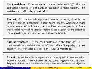


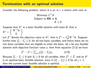
![3. Basic Feasible Solutions
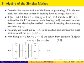
Consider the system Ax = b and x ≥ 0, where A is an m × n matrix
and b is any m vector.
Suppose that the rank(A, b) = rank(A) = m. After possibly
rearrangement of the columns of A, let A = [B, N] where B is an
m × m invertible matrix and N is m × (n − m) matrix.
The point X =
XB
XN
, where XB = B−1b and XN = 0 is called a
basic solution of the system.
If XB ≥ 0, then X is called a basic feasible solution of the system.
Here B is called the basic matrix (or simply the basis ) and N is
called the non basic matrix.
The components of XB are called basic variables, and the
components XN are called non basic variables.
If XB > 0, then X is called a non degenerate basic feasible
solution and if at least one component of XB is zero, then X is called
a degenerate basic feasible solution.
(Department of Mathematics Debark University )Linear Optimization(MATH 2062) October 7, 2020 12 / 107](https://image.slidesharecdn.com/chapter4simplexppt-201007055346/85/Chapter-4-Simplex-Method-ppt-12-320.jpg)
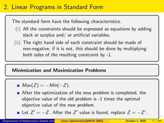
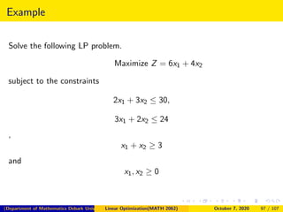
![Solution
(a) By introducing the slack variables x3 and x4 , the problem is put in the
following standard format:
x1 + x2 + x3 = 6
x2 + x4 = 3
x1, x2, x3, x4 ≥ 0
Note that, the constraint matrix
A = [a1 a2 a3 a4] =
1 1 1 0
0 1 0 1
From forgoing definition, basic feasible solutions corresponding to finding
a 2 × 2 basic matrix B with non-negative B−1b. The following are possible
ways of extracting B out of A.
(Department of Mathematics Debark University )Linear Optimization(MATH 2062) October 7, 2020 14 / 107](https://image.slidesharecdn.com/chapter4simplexppt-201007055346/85/Chapter-4-Simplex-Method-ppt-14-320.jpg)
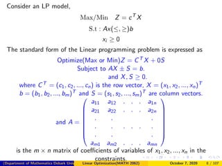
![B = [a1, a2] =
1 1
0 1
XB =
x1
x2
= B−1b =
1 −1
0 1
6
3
=
3
3
XN =
x3
x4
=
0
0
B = [a1, a4] =
1 0
0 1
XB =
x1
x4
= B−1b =
1 0
0 1
6
3
=
6
3
XN =
x2
x3
=
0
0
B = [a2, a3] =
1 1
1 0
XB =
x2
x3
= B−1b =
0 1
1 −1
6
3
=
3
3
XN =
x1
x4
=
0
0
(Department of Mathematics Debark University )Linear Optimization(MATH 2062) October 7, 2020 15 / 107](https://image.slidesharecdn.com/chapter4simplexppt-201007055346/85/Chapter-4-Simplex-Method-ppt-15-320.jpg)
![B = [a2, a4] =
1 0
1 1
XB =
x2
x4
= B−1b =
1 0
−1 1
6
3
=
6
−3
XN =
x1
x3
=
0
0
B = [a3, a4] =
1 0
0 1
XB =
x3
x4
= B−1b =
1 0
0 1
6
3
=
6
3
XN =
x1
x2
=
0
0
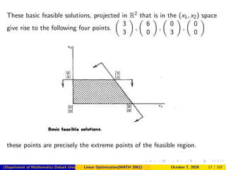
We have four basic feasible solutions.
Namely X1 =
3
3
0
0
, X2 =
6
0
0
3
, X3 =
0
3
3
0
, X4 =
0
0
6
3
(Department of Mathematics Debark University )Linear Optimization(MATH 2062) October 7, 2020 16 / 107](https://image.slidesharecdn.com/chapter4simplexppt-201007055346/85/Chapter-4-Simplex-Method-ppt-16-320.jpg)

![Example 2: Degenerate basic feasible solutions
Consider the following system of inequalities
x1 + x2 ≤ 6
x2 ≤ 3
x1 + 2x2 ≤ 9
x1, x2 ≥ 0
Solution: After adding the slack variables x3, x4 and x5, we get
x1 + x2 + x3 = 6
x2 + x4 = 3
x1 + 2x2 + x5 = 9
x1, x2, x3, x4, x5 ≥ 0
A = [a1, a2, a3, a4, a5] =
1 1 1 0 0
0 1 0 1 0
1 2 0 0 1
(Department of Mathematics Debark University )Linear Optimization(MATH 2062) October 7, 2020 20 / 107](https://image.slidesharecdn.com/chapter4simplexppt-201007055346/85/Chapter-4-Simplex-Method-ppt-20-320.jpg)
![Let us consider the basic feasible solution for B = [a1, a2, a3]
XB =
x1
x2
x3
=
1 1 1
0 1 0
1 2 0
−1
6
3
9
=
0 −2 1
0 1 0
1 1 −1
6
3
9
=
3
3
0
, XN =
x4
x5
=
0
0
Note that this basic feasible solution is degenerate since the basic variable
x3 = 0.
Now consider the basic feasible solution with B = [a1, a2, a4]
XB =
x1
x2
x4
=
1 1 0
0 1 1
1 2 0
−1
6
3
9
=
2 0 −1
−1 0 1
1 1 −1
6
3
9
=
3
3
0
, XN =
x3
x5
=
0
0
(Department of Mathematics Debark University )Linear Optimization(MATH 2062) October 7, 2020 21 / 107](https://image.slidesharecdn.com/chapter4simplexppt-201007055346/85/Chapter-4-Simplex-Method-ppt-21-320.jpg)
![Note that these basic feasible solution give rise to the same point obtained
by B = [a1, a2, a3]. It can be also checked the other basic feasible solution
with basis B = [a1, a2, a5] is give by
XB =
x1
x2
x5
=
3
3
0
, XN =
x3
x4
=
0
0
Note that all the three foregoing bases represent the single extreme point
or basic feasible solution (x1, x2, x3, x4, x5) = (3, 3, 0, 0, 0). This basic
feasible solution is degenerate since each associated basis involves a basic
variable at level zero.
(Department of Mathematics Debark University )Linear Optimization(MATH 2062) October 7, 2020 22 / 107](https://image.slidesharecdn.com/chapter4simplexppt-201007055346/85/Chapter-4-Simplex-Method-ppt-22-320.jpg)

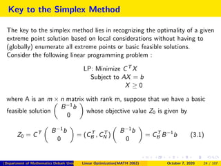


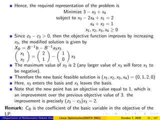
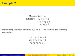
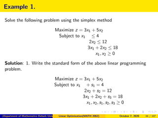
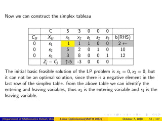
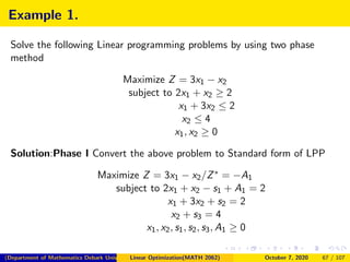
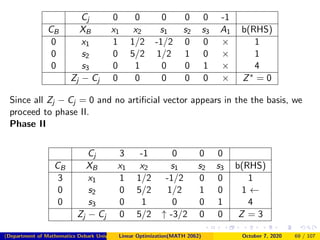
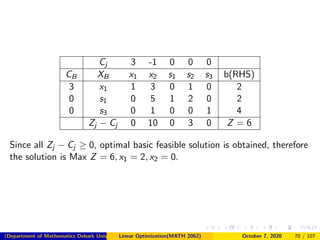
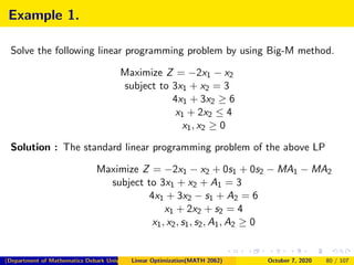
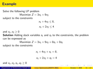
![Example 1.
Minimize x1 + x2
subject to x1 + 2x2 ≤ 4
x2 ≤ 1
x1, x2 ≥ 0
Solution: Introducing the slack variables x3 and x4 to put the problem in
a standard form.
This leads to the following constraint matrix A :
A = [a1, a2, a3, a4] =
1 2 1 0
0 1 0 1
Consider the basic feasible solution corresponding to B = [a1, a2].
In other words, x1 and x2 are the basic variables, while x3 and x4 are
the nonbasic variables.
The representation of the problem in this nonbasic variable space as
in Equation (3.4) with J= 3, 4 may be obtained as follows.
(Department of Mathematics Debark University )Linear Optimization(MATH 2062) October 7, 2020 31 / 107](https://image.slidesharecdn.com/chapter4simplexppt-201007055346/85/Chapter-4-Simplex-Method-ppt-31-320.jpg)
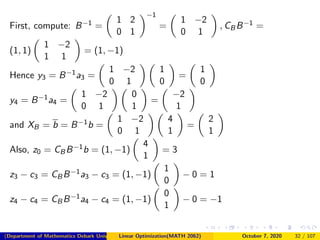
![Consider the basic feasible solution with basis
B = [a1, a2] =
−1 1
2 1
andB−1 =
−1/3 1/3
2/3 1/3
XB = B−1b − B−1NXN
xB1
xB2
=
x1
x2
=
−1/3 1/3
2/3 1/3
2
6
−
−1/3 1/3
2/3 1/3
1 0
0 1
x3
x4
=
4/3
10/3
−
−1/3
2/3
x3 −
1/3
1/3
x4 (3.10) Currently,
x3 = x4 = 0, x1 = 4/3 and x2 = 10/3, note that
z3 − c3 = CBB−1a3 − c3 =
(2, −1)
−1/3 1/3
2/3 1/3
1
0
− 0 = −4/3 0
1
0
− 0 = −4/3
z4 − c4 = CBB−1a4 − c4 = (2, −1)
−1/3 1/3
2/3 1/3
0
1
− 0 = 1/3
(Department of Mathematics Debark University )Linear Optimization(MATH 2062) October 7, 2020 36 / 107](https://image.slidesharecdn.com/chapter4simplexppt-201007055346/85/Chapter-4-Simplex-Method-ppt-36-320.jpg)


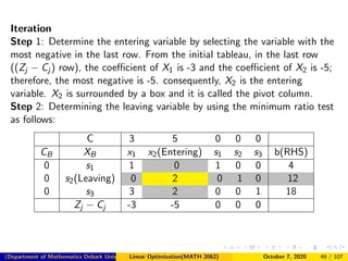
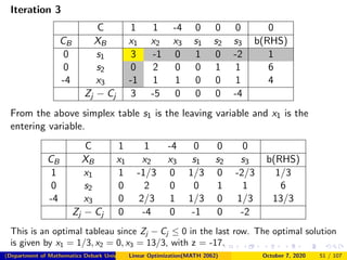
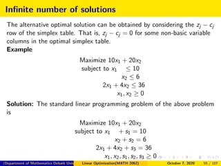
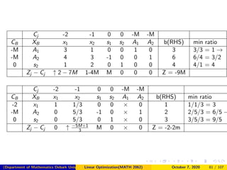
![Since b ≥ 0, then we can choose our initial basis as B = [a4, a5, a6] = I3,
and we indeed have B−1b = b ≥ 0. This gives the following initial tableau:
Iteration 1
C 1 1 -4 0 0 0 0
CB XB x1 x2 x3 s1 s2 s3 b(RHS)
0 s1 1 1 2 1 0 0 9
0 s2 1 1 -1 0 1 0 2
0 s3 -1 1 1 0 0 1 4
Zj − Cj -1 -1 4 0 0 0
The initial basic feasible solution in the above table is
x1 = 0, x2 = 0, x3 = 0, but it is not optimal, since there is positive element
the last row of the simplex table (Zj − Cj ). Identify the entering and
leaving variable
(Department of Mathematics Debark University )Linear Optimization(MATH 2062) October 7, 2020 49 / 107](https://image.slidesharecdn.com/chapter4simplexppt-201007055346/85/Chapter-4-Simplex-Method-ppt-49-320.jpg)
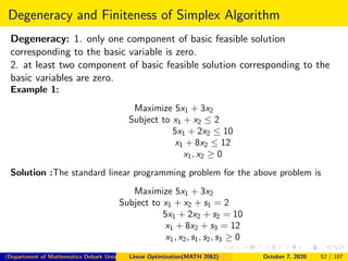
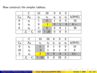
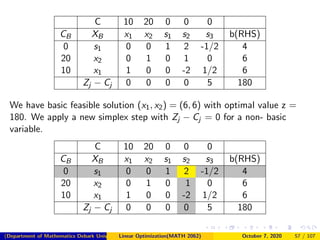
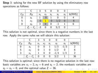
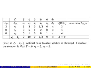
![C 10 20 0 0 0
CB XB x1 x2 s1 s2 s3 b(RHS)
0 s2 0 0 1/2 1 -1/4 2
20 x2 0 1 -1/2 0 1/4 4
10 x1 1 0 1 0 0 10
Zj − Cj 0 0 0 0 5 180
Now we have another basic solution (x1, x2) = (10, 4), but the optimal
values remains 180.
In our case, since (x1, x2) = (6, 6) and (x1, x2) = (10, 4) are solutions all
points of the segment (x1, x2)(x1, x2) = λ(6, 6) + (1 − λ)(10, 4), λ ∈ [0, 1]
are solutions.
(Department of Mathematics Debark University )Linear Optimization(MATH 2062) October 7, 2020 58 / 107](https://image.slidesharecdn.com/chapter4simplexppt-201007055346/85/Chapter-4-Simplex-Method-ppt-58-320.jpg)
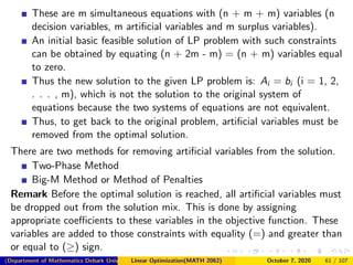
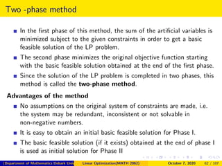
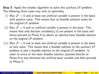
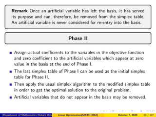
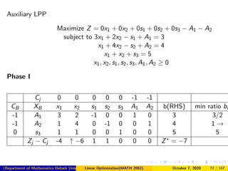
![Finding a Starting Basic Feasible Solution
In certain cases, it is difficult to obtain an initial basic feasible solution of
the given LP problem. Such cases arise
1 when the constraints are of the ≤ type,
n
j=1
aij xj ≤ bi , xj ≥ 0
and value of few right-hand side constants is negative [i.e. bi < 0].
After adding the non-negative slack variable si (i = 1, 2, . . ., m), the
initial solution so obtained will be si = −bi for a particular resource, i.
This solution is not feasible because it does not satisfy non-negativity
conditions of slack variables (i.e. si ≥ 0).
2 when the constraints are of the ≥ type,
n
j=1
aij xj ≥ bi , xj ≥ 0
(Department of Mathematics Debark University )Linear Optimization(MATH 2062) October 7, 2020 59 / 107](https://image.slidesharecdn.com/chapter4simplexppt-201007055346/85/Chapter-4-Simplex-Method-ppt-59-320.jpg)


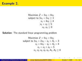


This document provides an overview of Chapter 4 on the Simplex Method for solving linear programming problems. It begins with an introduction to the simplex method and its development by George Dantzig. The chapter outline lists topics like linear programs in standard form, basic feasible solutions, and the simplex algorithm. It then discusses concepts such as slack and surplus variables, and conditions for applying the simplex method. Examples are provided to demonstrate converting problems to standard form and finding basic feasible solutions. The summary provides a high-level view of the key topics and concepts covered in the chapter on using the simplex method to solve linear programs.


![Human Reproduction [ Reproductive System ] Notes @irfanullah_mehar Irfanullah...](https://cdn.slidesharecdn.com/ss_thumbnails/humanreproductionreproductivesystemnotesirfanullahmeharirfanullahmeharjanantantra-260111172350-56e85778-thumbnail.jpg?width=640&height=640&fit=bounds)


