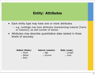
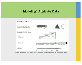
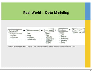
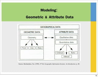
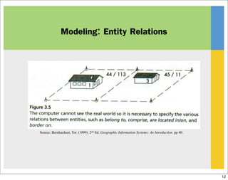
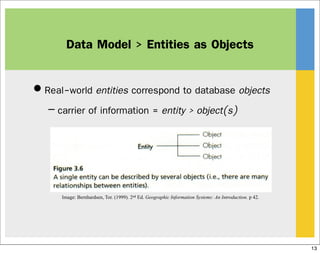
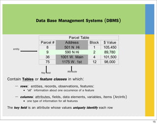
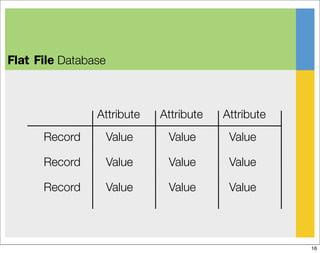
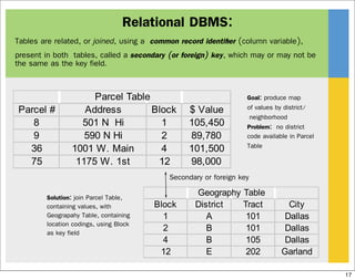
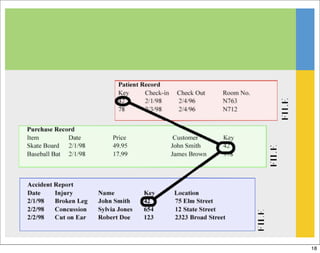
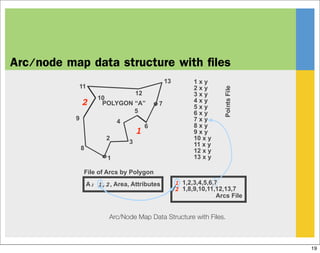
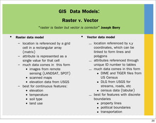
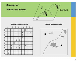
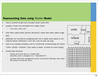
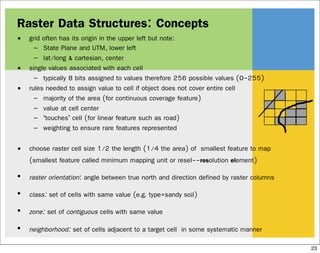
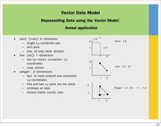
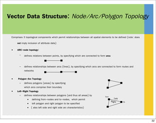
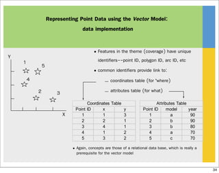
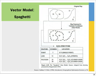
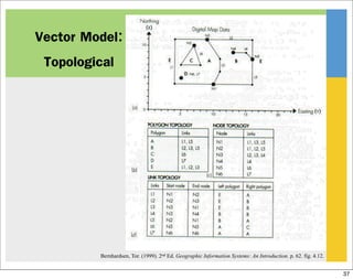
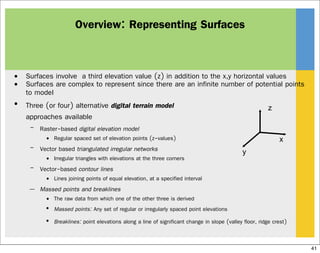
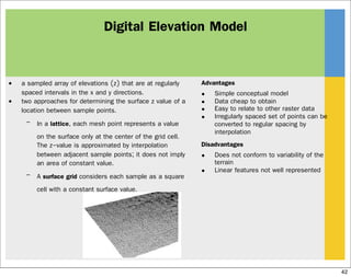
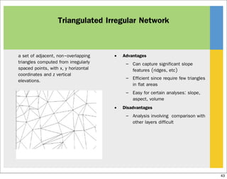
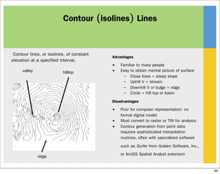
This document discusses how geographic features are represented in GIS data structures. Spatial data represents the location of features, while attribute data describes characteristics. Features can be represented using vector or raster data models. Vector models store location data as x,y coordinates and connect them to form lines and polygons. Raster models divide space into a grid of cells and store a single value for each cell. Relational databases are commonly used to organize spatial and attribute data for GIS analysis and mapping.

1. GIS Data Structures
1

2. Representing Geographic Features:
เราอธิบาย geographical features อยางไร?
• โดยอธิบายในรูปแบบของข้อมูลสองแบบ คือ:
– Spatial data ซึ่งอธิบายตำแหน่งที่ตั้ง (where)
– Attribute data ซึ่งอธิบายลักษณะของสิ่งที่เกิดขึ้น ณ ที่ตั้งนั้น
(what, how much, and when)
เราแสดงขอมูลใน GIS เปนดิจิตอลอยางไร?
• โดยการจัดให้เป็น layers ตามลักษณะของข้อมูลเกี่ยวกับ geographical features (เช่น hydrography, elevation,
water lines, sewer lines, grocery sales) โดยใช้:
– vector data model (coverage in ARC/INFO, shapefile in ArcView)
– raster data model (GRID or Image in ARC/INFO & ArcView)
• โดยจัดลักษณะของ data properties ในแต่ละ layer ให้สอดคล้องกับ:
– projection, scale, accuracy, and resolution
เรานำขอมูลตางๆ เขามาในระบบโปรแกรมในคอมพิวเตอรอยางไร?
• ใช้ความสามารถของระบบ GIS ที่สามารถจัดระบบฐานข้อมูลแบบ relational Data Base Management System
(DBMS)
2

3. Real World > Data Needed
• Basic carrier of information = entity
– Real-world phenomenon not divisible into phenomena of the
same kind
• An entity consists of:
– Type Classification
– Attributes
– Relationships
3

4. Entity: Type Classification
 Assumes identical occurrences can be classified
 Each entity type must be unique (no ambiguity)
– e.g., detached house classified under house; not industrial building
 Some entities may need to be categorized
– e.g., roadways as a class: with categories for national highways, urban
roads, private roads
 Entity type also known as qualitative data
– or in statistics the ‘nominal scale’
4

5. Entity: Attributes
• Each entity type may have one or more attributes
– e.g., buildings may have attributes characterizing material (frame
or masonry), as well number of stories
• Attributes may describe quantitative data ranked in three
levels of accuracy
Ordinal (Ranks)
– Good
– Better
– Best
Interval (numeric)
– Age
– Income
Ratio (scale)
– Length
– Area
5

6. Spatial Data Types
• continuous: elevation, rainfall, ocean salinity
• areas:
– unbounded: landuse, market areas, soils, rock type
– bounded: city/county/state boundaries, ownership parcels, zoning
– moving: air masses, animal herds, schools of fish
• networks: roads, transmission lines, streams
• points:
– fixed: wells, street lamps, addresses
– moving: cars, fish, deer
6

7. Attribute data types
Categorical (name):
– nominal
• no inherent ordering เช่น land use
types, county names
– ordinal
• inherent order เช่น road class;
stream class
• บางครั้งก็แสดงเป็นตัวเลขที่ถือเป็นเพียงแค่
ชื่อเฉพาะ ไม่นำไปใช้ในการคำนวณ
Numerical
Known difference between values
– interval
• No natural zero
• can’t say ‘twice as much’
• temperature (Celsius or
Fahrenheit)
– ratio
• natural zero
• ratios make sense (e.g. twice as
much)
• income, age, rainfall
• ค่าตัวเลขเป็นเลขเต็ม integer [whole number]
or หรือจุดทศนิยม floating point [decimal
fraction]
7

8. Real World > Data Modeling
Source: Bernhardsen, Tor. (1999). 2nd Ed. Geographic Information Systems: An Introduction. p 38.
8

9. Real World >
Modeling
Process
Source: Bernhardsen, Tor. (1999). 2nd Ed.
Geographic Information Systems: An
Introduction. p 39. Fig 3.2.
9

10. Modeling:
Geometric & Attribute Data
Source: Bernhardsen, Tor. (1999). 2nd Ed. Geographic Information Systems: An Introduction. p. 40.
10

11. Modeling: Attribute Data
Source: Bernhardsen, Tor. (1999). 2nd Ed. Geographic Information Systems: An Introduction. pp 40.
11

12. Modeling: Entity Relations
Source: Bernhardsen, Tor. (1999). 2nd Ed. Geographic Information Systems: An Introduction. pp 40.
12

13. Data Model > Entities as Objects
 Real-world entities correspond to database objects
– carrier of information = entity > object(s)
Image: Bernhardsen, Tor. (1999). 2nd Ed. Geographic Information Systems: An Introduction. p 42.
13

14. Objects Characterized by:
• Type (unique ID, type code/object class)
• Attributes (qualitative/quantitative data)
• Relations (calculable vs. attributable)
• Geometry (point, line, area/polygon)
• Quality (accuracy, resolution, coverage extent,
representation, etc.)
14

15. Data Base Management Systems (DBMS)
Contain Tables or feature classes in which:
– rows: entities, records, observations, features:
• ‘all’ information about one occurrence of a feature
– columns: attributes, fields, data elements, variables, items (ArcInfo)
• one type of information for all features
The key field is an attribute whose values uniquely identify each row
entity
AttributeKey field
15

16. Flat File Database
Record Value Value Value
Attribute Attribute Attribute
Record Value Value Value
Record Value Value Value
16

17. Relational DBMS:
Goal: produce map
of values by district/
neighborhood
Problem: no district
code available in Parcel
Table
Solution: join Parcel Table,
containing values, with
Geograpahy Table, containing
location codings, using Block
as key field
Tables are related, or joined, using a common record identifier (column variable),
present in both tables, called a secondary (or foreign) key, which may or may not be
the same as the key field.
Secondary or foreign key
17

18. 18

19. Arc/node map data structure with files
Arc/Node Map Data Structure with Files.
1 1,2,3,4,5,6,7
Arcs File
POLYGON “A”
A: 1,2, Area, Attributes
File of Arcs by Polygon
1
2
3
4
5
6
7
8
9
10
11
12
13 1 x y
2 x y
3 x y
4 x y
5 x y
6 x y
7 x y
8 x y
9 x y
10 x y
11 x y
12 x y
13 x y
PointsFile
1
2
2 1,8,9,10,11,12,13,7
19

20. GIS Data Models:
Raster v. Vector
“raster is faster but vector is corrector” Joseph Berry
• Raster data model
– location is referenced by a grid
cell in a rectangular array
(matrix)
– attribute is represented as a
single value for that cell
– much data comes in this form
• images from remote
sensing (LANDSAT, SPOT)
• scanned maps
• elevation data from USGS
– best for continuous features:
• elevation
• temperature
• soil type
• land use
• Vector data model
– location referenced by x,y
coordinates, which can be
linked to form lines and
polygons
– attributes referenced through
unique ID number to tables
– much data comes in this form
• DIME and TIGER files from
US Census
• DLG from USGS for
streams, roads, etc
• census data (tabular)
– best for features with discrete
boundaries
• property lines
• political boundaries
• transportation
20

21. Real World
Vector RepresentationRaster Representation
Concept of
Vector and Raster
line
polygon
point
21

22. Representing Data using Raster Model
• area is covered by grid with (usually) equal-sized cells
• location of each cell calculated from origin of grid:
– “two down, three over”
• cells often called pixels (picture elements); raster data often called image
data
• attributes are recorded by assigning each cell a single value based on the
majority feature (attribute) in the cell, such as land use type.
• easy to do overlays/analyses, just by ‘combining’ corresponding cell values:
“yield= rainfall + fertilizer” (why raster is faster, at least for some things)
• simple data structure:
– directly store each layer as a single table
(basically, each is analagous to a “spreadsheet”)
– computer data base management system not required (although many raster
GIS systems incorporate them)
corn
wheat
fruit
clover
fruit
oats
0 1 2 3 4 5 6 7 8 9
0
1
2
3
4
5
6
7
8
9
1 1 1 1 1 4 4 5 5 5
1 1 1 1 1 4 4 5 5 5
1 1 1 1 1 4 4 5 5 5
1 1 1 1 1 4 4 5 5 5
1 1 1 1 1 4 4 5 5 5
2 2 2 2 2 2 2 3 3 3
2 2 2 2 2 2 2 3 3 3
2 2 2 2 2 2 2 3 3 3
2 2 4 4 2 2 2 3 3 3
2 2 4 4 2 2 2 3 3 3
22

23. • grid often has its origin in the upper left but note:
– State Plane and UTM, lower left
– lat/long & cartesian, center
• single values associated with each cell
– typically 8 bits assigned to values therefore 256 possible values (0-255)
• rules needed to assign value to cell if object does not cover entire cell
– majority of the area (for continuous coverage feature)
– value at cell center
– ‘touches’ cell (for linear feature such as road)
– weighting to ensure rare features represented
• choose raster cell size 1/2 the length (1/4 the area) of smallest feature to map
(smallest feature called minimum mapping unit or resel--resolution element)
• raster orientation: angle between true north and direction defined by raster columns
• class: set of cells with same value (e.g. type=sandy soil)
• zone: set of contiguous cells with same value
• neighborhood: set of cells adjacent to a target cell in some systematic manner
Raster Data Structures: Concepts
23

24. Full Matrix--162 bytes
111111122222222223
111111122222222233
111111122222222333
111111222222223333
111113333333333333
111113333333333333
111113333333333333
111333333333333333
111333333333333333
1,7,2,17,3,18
1,7,2,16,3,18
1,7,2,15,3,18
1,6,2,14,3,18
1,5,3,18
1,5,3,18
1,5,3,18
1,3,3,18
1,3,3,18
Raster Data Structures
Runlength Compression (for single layer)
Run Length (row)--44 bytes
“Value thru column” coding.
1st number is value, 2nd is
last column with that value.
Now, GIS packages generally rely on commercial
compression routines. Pkzip is the most common,
general purpose routine. MrSid (from Lizard
Technology)and ECW (from ER Mapper) are used
for images. All these essentially use the same
concept. Occasionally, data is still delivered to you
in run-length compression, especially in remote
sensing applications.
This is a “lossless”
compression, as
opposed to “lossy,”
since the original
data can be exactly
reproduced.
24

25. Raster Data Structures
Quad Tree Representation (for single layer)
• sides of square grid divided evenly on a
recursive basis
– length decreases by half
– # of areas increases fourfold
– area decreases by one fourth
• Resample by combining (e.g. average) the
four cell values
– although storage increases if save all
samples, can save processing costs
if some operations don’t need high
resolution
• for nominal or binary data can save
storage by using maximum block
representation
– all blocks with same value at any one
level in tree can be stored as single
value
store this quadrant
as single 1
store this quadrant
as single zero
1 1
1 1
1 1
1
1
I 1,0,1,1 II 1
III 0,0,0,1 IV 0
Essentially involves compression applied to both row and column.
2
2
1
2
3
4
4
4
4
54
4
4
3
4
2
3 4
2.5
3.5
3.25
25

26. Raster Data Structures:
Raster Array Representations for multiple layers
• raster data comprises rows and columns, by
one or more characteristics or arrays
– elevation, rainfall, & temperature; or multiple
spectral channels (bands) for remote sensed
data
– how organise into a one dimensional data
stream for computer storage & processing?
• Band Sequential (BSQ)
– each characteristic in a separate file
– elevation file, temperature file, etc.
– good for compression
– good if focus on one characteristic
– bad if focus on one area
• Band Interleaved by Pixel (BIP)
– all measurements for a pixel grouped together
– good if focus on multiple characteristics of
geographical area
– bad if want to remove or add a layer
• Band Interleaved by Line (BIL)
– rows follow each other for each characteristic
A B
B B
III IV
I II 150 160
120 140
Elevation
Soil
Veg
File 1: Veg A,B,B,B
File 2: Soil I,II,III,IV
File 3: El. 120,140,150,160
A,I,120, B,II,140 B,III,150 B,IV,160
A,B,I,II,120,140 B,B,III,IV,150,160
Note that we start in lower left.
Upper left is alternative.
26

27. Vector Data Model
Representing Data using the Vector Model:
formal application
• point (node): 0-dimension
– single x,y coordinate pair
– zero area
– tree, oil well, label location
• line (arc): 1-dimension
– two (or more) connected x,y
coordinates
– road, stream
• polygon : 2-dimensions
– four or more ordered and connected
x,y coordinates
– first and last x,y pairs are the same
– encloses an area
– census tracts, county, lake
Point: 7,2
Line: 7,2 8,1
Polygon: 7,2 8,1 7,1 7,2
8
.
x=7
y=2
1
2
7
1
2
7
1
2
7 8
8
27

28. Vector Data Structures:
Whole Polygon
Whole Polygon (boundary structure): polygons described by listing coordinates of points in order as you ‘walk
around’ the outside boundary of the polygon.
– all data stored in one file
• could also store--inefficiently--attribute data for polygon in same file
– coordinates/borders for adjacent polygons stored twice;
• may not be same, resulting in slivers (gaps), or overlap
• how assure that both updated?
– all lines are ‘double’ (except for those on the outside periphery)
– no topological information about polygons
• which are adjacent and have common boundary?
• how relate different geographies? e.g. zip codes and tracts?
– used by the first computer mapping program, SYMAP, in late ‘60s
– adopted by SAS/GRAPH and many business thematic mapping programs.
Topology
--knowledge about
relative spatial
positioning
--managing data
cognizant of shared
geometry
Topography!
--the form of the land
surface, in particular, its
elevation
28

29. Whole Polygon:
illustration
A 3 4
A 4 4
A 4 2
A 3 2
A 3 4
B 4 4
B 5 4
B 5 2
B 4 2
B 4 4
C 3 2
C 4 2
C 4 0
E A B
C D
1 2 3 4 5
0
1
2
3
4
5 C 3 0
C 3 2
D 4 2
D 5 2
D 5 0
D 4 0
D 4 2
E 1 5
E 5 5
E 5 4
E 3 4
E 3 0
E 1 0
E 1 5
Data File
29

30. Vector Data Structures:
Points & Polygons
Points and Polygons: polygons described by listing ID numbers of points
in order as you ‘walk around the outside boundary’; a second file
lists all points and their coordinates.
– solves the duplicate coordinate/double border problem
– lines can be handled similar to polygons (list of IDs) , but how handle
networks?
– still no topological information
– first used by CALFORM, the second generation mapping package, from the
Laboratory for Computer Graphics and Spatial Analysis at Harvard in early
‘70s
30

31. Points and Polygons:
Illustration
1 3 4
2 4 4
3 4 2
4 3 2
5 5 4
6 5 2
7 5 0
8 4 0
9 3 0
10 1 0
11 1 5
12 5 5
E A B
C D
1 2 3 4 5
0
1
2
3
4
5 A 1, 2, 3, 4, 1
B 2, 5, 6, 3, 2
C 4, 3, 8, 9, 4
D 3, 6, 7, 8, 3
E 11, 12, 5, 1, 9, 10, 11
Points File
1
2
34
5
6
78910
11
12
Polygons File
31

32. Comprises 3 topological components which permit relationships between all spatial elements to be defined (note: does
not imply inclusion of attribute data)
• ARC-node topology:
– defines relations between points, by specifying which are connected to form arcs
– defines relationships between arcs (lines), by specifying which arcs are connected to form routes and
networks
• Polygon-Arc Topology
– defines polygons (areas) by specifying
which arcs comprise their boundary
• Left-Right Topology
– defines relationships between polygons (and thus all areas) by
• defining from-nodes and to-nodes, which permit
• left polygon and right polygon to be specified
• ( also left side and right side arc characteristics)
Vector Data Structure: Node/Arc/Polygon Topology
Left
Right
from
to
32

33. Node/Arc/ Polygon and Attribute Data
Relational Representation: DBMS required!
Spatial Data Attribute Data
Birch
Cherry
I
II
III
IV
1
4 3
A35
Smith
Estate A34
2
33

34. 1
2 3
4
5
X
Representing Point Data using the Vector Model:
data implementation
Y
• Features in the theme (coverage) have unique
identifiers--point ID, polygon ID, arc ID, etc
• common identifiers provide link to:
– coordinates table (for ‘where)
– attributes table (for what)
• Again, concepts are those of a relational data base, which is really a
prerequisite for the vector model
34

35. Variety of Vector Models
• Spaghetti model
• Topological model (most common)
• Triangulated irregular network (TIN)
• Dime files and TIGER files
• Network model
• Digital Line Graph (DLG)
• Shapefile (ArcView/ArcGIS; ESRI)
• Others: HPGL, PostScript/ASCII, CAD/.dxf
35

36. Vector Model:
Spaghetti
Source: Lakhan, V. Chris. (1996). Introductory Geographical Information Systems. p. 54.
36

37. Vector Model:
Topological
Bernhardsen, Tor. (1999). 2nd Ed. Geographic Information Systems: An Introduction. p. 62. fig. 4.12.
37

38. Why Topology Matters
• Connections & relationships between objects are
independent of their coordinates
• Overcomes major weakness of spaghetti model – allowing
for GIS analysis (Overlaying, Network, Contiguity,
Connectivity)
• Requires all lines be connected, polygons closed, loose ends
removed.
38

39. Vector Model: Network
Source: Heywood, Ian and Sarah Cornelius and Steve Carver. An Introduction to Geographical Information Systems. p. 60. fig. 3.14.
39

40. Vector Model:
TIN: Triangulated Irregular Network Surface
A B
CD
6
1
2
3
4
5
E
F
G
H
Elevation points (nodes)
chosen based on relief
complexity, and then their 3-
D location (x,y,z) determined.
Points
Elevation points connected to
form a set of triangular
polygons; these then
represented in a vector
structure.
Polygons Attribute Info. Database
Attribute data associated
via relational DBMS (e.g.
slope, aspect, soils, etc.)
Advantages over raster:
•fewer points
•captures discontinuities (e.g ridges)
•slope and aspect easily recorded
Disadvantages: Relating to other polygons for map
overlay is compute intensive (many polygons)
40

41. Overview: Representing Surfaces
• Surfaces involve a third elevation value (z) in addition to the x,y horizontal values
• Surfaces are complex to represent since there are an infinite number of potential points
to model
• Three (or four) alternative digital terrain model
approaches available
– Raster-based digital elevation model
• Regular spaced set of elevation points (z-values)
– Vector based triangulated irregular networks
• Irregular triangles with elevations at the three corners
– Vector-based contour lines
• Lines joining points of equal elevation, at a specified interval
– Massed points and breaklines
• The raw data from which one of the other three is derived
• Massed points: Any set of regular or irregularly spaced point elevations
• Breaklines: point elevations along a line of significant change in slope (valley floor, ridge crest)
x
y
z
41

42. Digital Elevation Model
• a sampled array of elevations (z) that are at regularly
spaced intervals in the x and y directions.
• two approaches for determining the surface z value of a
location between sample points.
– In a lattice, each mesh point represents a value
on the surface only at the center of the grid cell.
The z-value is approximated by interpolation
between adjacent sample points; it does not imply
an area of constant value.
– A surface grid considers each sample as a square
cell with a constant surface value.
Advantages
• Simple conceptual model
• Data cheap to obtain
• Easy to relate to other raster data
• Irregularly spaced set of points can be
converted to regular spacing by
interpolation
Disadvantages
• Does not conform to variability of the
terrain
• Linear features not well represented
42

43. Triangulated Irregular Network
• Advantages
– Can capture significant slope
features (ridges, etc)
– Efficient since require few triangles
in flat areas
– Easy for certain analyses: slope,
aspect, volume
• Disadvantages
– Analysis involving comparison with
other layers difficult
a set of adjacent, non-overlapping
triangles computed from irregularly
spaced points, with x, y horizontal
coordinates and z vertical
elevations.
43

44. Contour (isolines) Lines
Advantages
• Familiar to many people
• Easy to obtain mental picture of surface
– Close lines = steep slope
– Uphill V = stream
– Downhill V or bulge = ridge
– Circle = hill top or basin
Disadvantages
• Poor for computer representation: no
formal digital model
• Must convert to raster or TIN for analysis
• Contour generation from point data
requires sophisticated interpolation
routines, often with specialized software
such as Surfer from Golden Software, Inc.,
or ArcGIS Spatial Analyst extensionridge
valley hilltop
Contour lines, or isolines, of constant
elevation at a specified interval,
44